Interface and model reduction for efficient explicit simulations - a case study with nonlinear vehicle crash models

Figures & data

Figure 1. Workflow of the process suggested to speed up explicit simulations. The new converters and procedures derived in the course of this research are the Binout-Reader, the LS-Dyna import and the d3eigv writer. Furthermore, the workflow shows how MatMorembs is used to calculate the reduced elastic body for the online simulation.

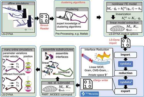
Figure 2. Race kart used as a simple surrogate vehicle model. The race kart consists of a frame, an engine next to the seat, a rear shaft, frontal steering components and tyres.

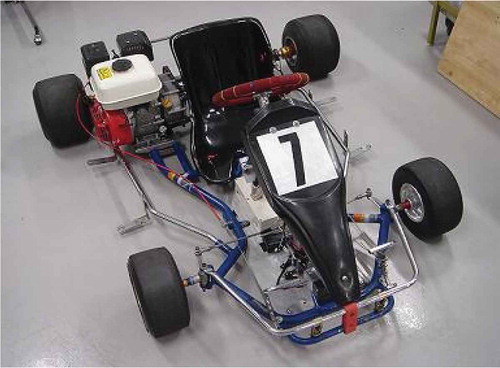
Figure 3. Main parts of the simulated crash scenario. The kart frame crashes into the rigid pole. Forces and moments represent the interactions between kart frame, tyres and rear shaft.

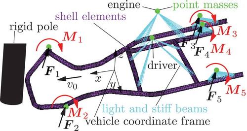
Figure 4. Kinematics of the original (unreduced) central crash with 32 km/h. The legend indicates the plastic strain.

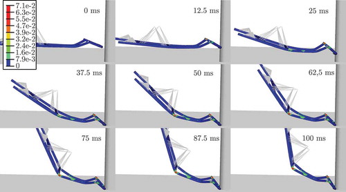
Figure 5. Initial condition of the offline simulations to determine areas with ‘linear’ and ‘nonlinear’ behaviour. The crash position of the pole is labelled with left, central and right.

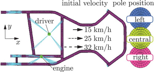
Figure 6. Frame cut into a frontal nonlinear described part and a rear linear described part.

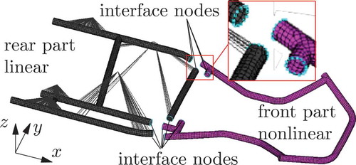
Figure 7. Acceleration of the driver for v₀ = 32 km/h, where left, central and right refer to the position of the pole.

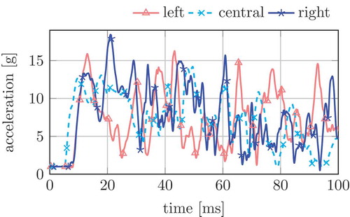
Figure 8. Final positions and effective plastic strains of the racing kart. The offline simulations are performed to determine linear and nonlinear behaviour of the kart. The rows of the figure represent the initial velocities v₀ and the columns represent the three different locations of the pole.

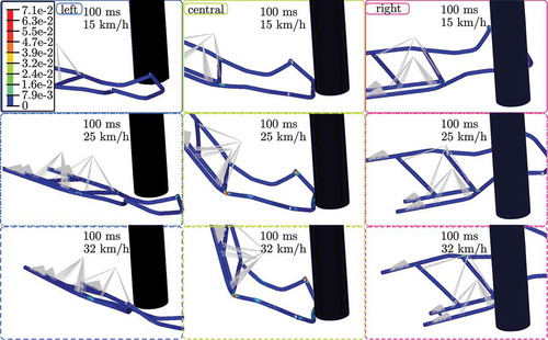
Table 1. Number of elements and nodes for the split model.

	Kart parts
	Front	Rear
# elements	4304	5727
# nodes	4244	5174
# DOF	25,464	31,044

Figure 9. Norm of the transfer matrix of full and reduced systems and the corresponding error measures.

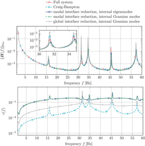
Figure 10. Acceleration of the driver for v₀ = 32 km/h in a central crash. The results are calculated with different simulation models where the reduced models are calculated with different reduction approaches.

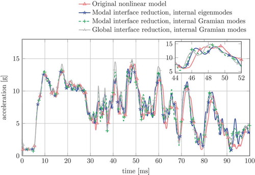
Figure 11. Plastic strain of the deformed reduced model (CMS-Gram with modal interface reduction) plus the kinematics of the unreduced model for the central crash.

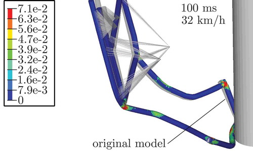
Table 2. Calculation times in LS-DYNA.

	Original		CB^[^1^]
	CMSG-IR^[^2^]
Elapsed time [10^3s]	3.9	3.75	3935
Element proc.^[^3^] [10^3s]	2.21	0.97	94.9
El. body proc.^[^4^] [10^3s]		1.26	3582
Problem cycles [10^6]	0.63	0.63	38.18
Mean time step [ns]	150	150	2

^[1] Standard Craig–Bampton;

^[2] CMS Gram with modal interface reduction;

^[3] Element processing;

^[4] Elastic body processing.