Balanced truncation model reduction for linear time-varying systems

Figures & data

Table

Algorithm 1 Balanced truncation for LTV systems.

Require: $(E(t),A(t),B(t),C(t))$

Ensure: a reduced-order system $(\hat{E}(t),\hat{A}(t),\hat{B}(t),\hat{C}(t))$

1: Compute the Cholesky factors $R(t)$ and $L(t)$ of the reachability and observability Gramians $P(t)=R(t)R^T(t)$ and $Q(t)=L(t)L^T(t)$ satisfying the DLEs (3) and (4), respectively.

2: Compute the singular value decomposition $R^T(t)E^T(t)L(t)=[\hspace{0.17em}{U}_1(t),\hspace{0.17em}{U}_2(t)\hspace{0.17em}]\left[\begin{array}{cc}{\mathrm{\Sigma }}_1(t)& \hspace{0.17em}\\ \hspace{0.17em}& {\mathrm{\Sigma }}_2(t)\end{array}\right][\hspace{0.17em}{V}_1(t),\hspace{0.17em}{V}_2(t)\hspace{0.17em}{]}^T,$

where the matrices $[\hspace{0.17em}{U}_1(t),\hspace{0.17em}{U}_2(t)\hspace{0.17em}]$ and $[\hspace{0.17em}{V}_1(t),\hspace{0.17em}{V}_2(t)\hspace{0.17em}]$ have orthonormal columns, ${\mathrm{\Sigma }}_1(t)=\mathrm{d}\mathrm{i}\mathrm{a}\mathrm{g}({\sigma }_1(t),\dots ,{\sigma }_r(t))$ and ${\mathrm{\Sigma }}_2(t)=\mathrm{d}\mathrm{i}\mathrm{a}\mathrm{g}({\sigma }_{r+1}(t),\dots ,{\sigma }_n(t))$.

3: Compute the reduced-order system (2) with (6) $\begin{array}{cc}\hat{E}(t)=W^T(t)E(t)Z(t),& \hat{A}(t)=W^T(t)(AZ(t)-E(t)\dot{Z}(t)),\\ \hat{B}(t)=W^T(t)B(t),& \hat{C}(t)=C(t)Z(t),\end{array}$(6)

where $W(t)=L(t)V_1(t){\mathrm{\Sigma }}_1^{-1/2}(t)$ and $Z(t)=R(t)U_1(t){\mathrm{\Sigma }}_1^{-1/2}(t)$.

Table 1. Coefficients of the $s$-step BDF method.

$s$	$\beta$	${\alpha }_0$	${\alpha }_1$	${\alpha }_2$	${\alpha }_3$	${\alpha }_4$	${\alpha }_5$	${\alpha }_6$
1	1	1	–1
2	2	3	–4	1
3	6	11	–18	9	–2
4	12	25	–48	36	–16	3
5	60	137	–300	300	–200	75	–12
6	60	147	–360	450	–400	225	–72	10

Table 2. Heated beam: the computation time for solving the DLE and the square root method.

Method		BDF1	BDF2	BDF3	BDF6	Ros1	Ros2
Time [s]	DLE	1 396.91	2 242.02	2 885.42	4 762.31	1 448.93	14 383.45
	SRM	0.93	1.04	1.33	2.53	1.06	2.79

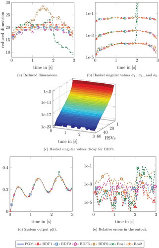
Figure 1. Heated beam: (a) dimensions of the reduced state at different times, (b) the Hankel singular values ${\sigma }_1$, ${\sigma }_3$ and ${\sigma }_6$ for the BDF methods of order $1$, $2$, $3$ and, $6$ and the Rosenbrock schemes of order $1$ and $2$, (c) Hankel singular values for the BDF method of order 1, (d) the outputs of the full and the reduced-order models and (e) relative errors in the output.

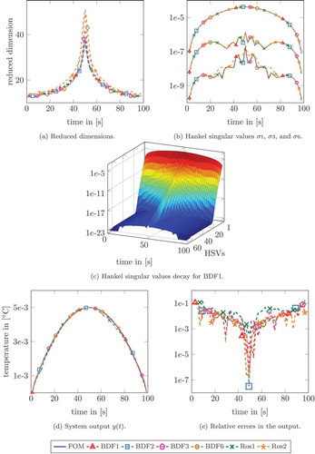
Table 3. Steel profile: the computation time for solving the DLE and the square root method.

Method		BDF1	BDF2	BDF3	BDF6	Ros1	Ros2
Time [s]	DLE	6 993.58	7 634.43	8 008.14	10 136.86	6 994.55	35 374.41
	SRM	6.15	8.83	7.46	12.56	6.37	13.71

Figure 2. Steel profile: (a) dimensions of the reduced state at different times, (b) the Hankel singular values ${\sigma }_1$, ${\sigma }_3$ and ${\sigma }_6$ for the BDF methods of order $1$, $2$, $3$ and $6$ and the Rosenbrock schemes of order $1$ and $2$, (c) Hankel singular values for the BDF method of order 1, (d) the outputs of the full and the reduced-order models and (e) relative errors in the output.

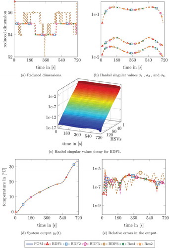
Table 4. Burgers equation: the computation time for solving the DLE and the square root method.

Method		BDF1	BDF2	BDF3	BDF6	Ros1	Ros2
Time [s]	DLE	4 389.66	3 893.65	3 917.39	4 808.24	4 378.24	17 862.08
	SRM	1.23	1.52	1.34	1.64	1.35	1.51

Figure 3. Burgers equation: (a) dimensions of the reduced state at different times, (b) the Hankel singular values ${\sigma }_1$, ${\sigma }_3$ and ${\sigma }_6$ for the BDF methods of order $1$, $2$, $3$ and $6$ and the Rosenbrock schemes of order $1$ and $2$, (c) Hankel singular values for the BDF method of order 1, (d) the outputs of the full and the reduced-order models and (e) relative errors in the output.