An empirical interpolation approach to reduced basis approximations for variational inequalities

Figures & data

Figure 1. Solutions u(x; μ) and the corresponding obstacles h(x; μ) of the first numerical example in Section 4.

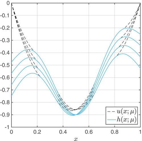
Figure 2. The first five basis vectors forming g_M’s space W_M in the numerical example for the barrier method in Section 4. The basis $\{q_i{\}}_{i=1}^5$ is constructed by EIM.

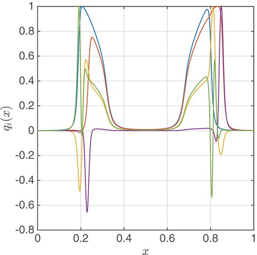
Figure 3. First five basis vectors forming the reduced basis space $W_N^u$ in the numerical example for the barrier method in Section 4. The basis $\{{\zeta }_i{\}}_{i=1}^5$ is constructed by greedy procedure based on the a posteriori error estimator (only the residual part $\epsilon$_NM).

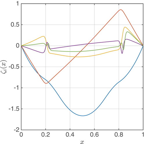
Figure 4. Relative convergence of barrier/exp-penalty solutions to the reference solution, depending on the homotopy parameter $\nu$, measured in V-norm.

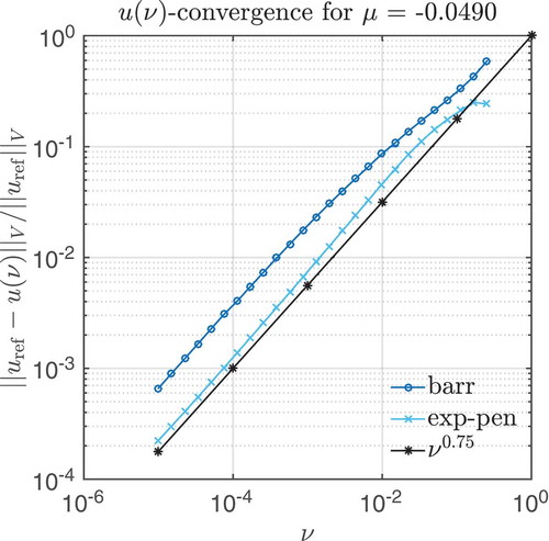
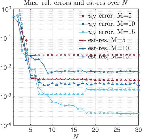
Figure 5. Barrier method: maximal relative error and estimator decay (only residual part) for different N, M values.

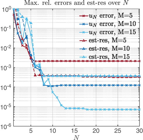
Figure 6. Exp-penalty method: maximal relative error and estimator decay (only residual part) for different N, M values.

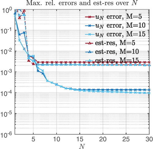
Figure 7. Barrier method: Numerical instabilities for the case when the homotopy parameter is very small ($\nu$_final = 1E – 4). Maximal relative error and estimator decay (only residual part) for different M, N values.

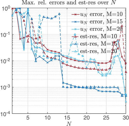
Figure 8. Exp-penalty method: Numerical instabilities the case when the homotopy parameter is very small ($\nu$_final = 1E – 4). Maximal relative error and estimator decay (only residual part) for different M, N values.

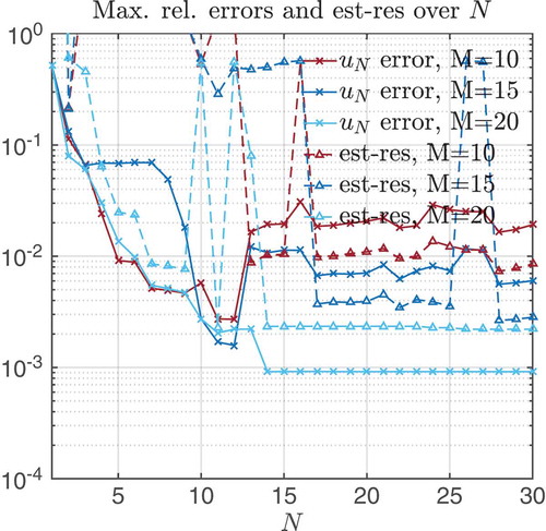
Table 1. Barrier method.

N	M	Max-err	Max-est	Max-est-res	Ave-eff (res)	Speed-up ratio
5	5	2.76E – 03	1.20E – 02	3.13E – 03	2.79E + 00	27.8
5	10	2.87E – 03	2.64E – 02	4.33E – 03	1.09E + 01	27.6
10	5	2.12E – 03	1.35E – 02	3.86E – 04	3.92E + 00	27.2
10	10	1.14E – 04	1.69E – 02	3.70E – 04	9.33E + 01	27.2
20	20	2.86E – 06	1.49E – 02	1.32E – 04	1.16E + 02	22.9
30	30	2.36E – 05	3.75E – 04	3.74E – 04	6.52E + 01	19.1

We display for certain N, M the following relative errors and relative estimators in the V-norm: maximal error, maximal estimator and maximal residual estimator. Further, we show the averaged effectivity $\bar{\eta }$ max-est-res and the speed-up ratio.

Table 2. Exp-penalty method.

N	M	Max-err	Max-est	Max-est-res	Ave-eff (res)	Speed-up ratio
5	5	4.63E – 03	1.16E – 01	2.37E – 03	2.46E + 01	17.5
5	10	5.47E – 03	9.14E – 03	3.26E – 03	2.73E + 00	17.3
10	5	2.92E – 03	1.15E – 01	2.26E – 03	3.61E + 01	17.5
10	10	2.45E – 04	5.06E – 03	2.22E – 03	1.91E + 01	17.3
20	20	1.12E – 04	2.13E – 03	2.13E – 03	1.72E + 01	15.3
30	30	9.63E – 05	2.05E – 03	2.05E – 03	2.05E + 01	13.1

We display for certain N, M the following relative errors and relative estimators in the V-norm: maximal error, maximal estimator and maximal residual estimator. Further, we show the averaged effectivity $\bar{\eta }$ of max-est-res and the speed-up ratio.

Table 3. Barrier method.

N	M	Max-err	Max-est	Max-est-res	Ave-eff (res)	Speed-up ratio
5	5	2.20E – 03	1.53E – 02	5.40E – 04	4.38E + 00	40
5	10	2.52E – 03	2.86E – 02	3.38E – 03	1.72E + 01	38.7
10	5	2.13E – 03	1.36E – 02	3.88E – 04	3.94E + 00	38.1
10	10	1.24E – 04	1.72E – 02	3.69E – 04	8.29E + 01	37.8
20	20	7.33E – 06	3.90E – 04	2.58E – 04	5.40E + 01	31.6
30	30	2.08E – 05	3.79E – 04	3.78E – 04	6.03E + 01	26.8

The same setting as for Figure 5 and Table 1 but instead of using 2 quadrature points we now use 5.

Figure 9. Solutions u(x; μ) and the corresponding obstacles h(x; μ) of the second numerical example; using the exp-penalty method ($\nu$_final = 1E – 3).

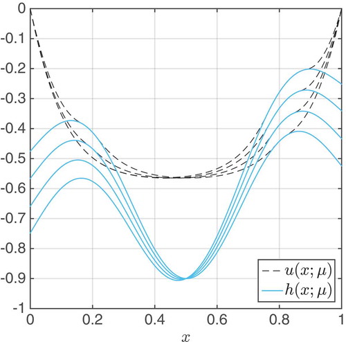
Figure 10. The exp-penalty method applied to a VI with non-linear f(∙): Maximal relative error and estimator decay (only residual part) for different N, M values.