Tangential interpolation-based eigensystem realization algorithm for MIMO systems

Figures & data

Algorithm 1. TERA

input: Markov parameters $h_1,h_2,\dots ,h_{2s-1}$;

Reduced model order $r$;

Number of tangential directions ${\mathrm{\ell }}_1,{\mathrm{\ell }}_2$ .

Output: State space realization $(A_r,B_r,C_r)$.

1: Compute svd: $[h_1{h}_2\cdots h_{2s-1}]=U\mathrm{\Sigma }{V}^T.$

2: $W_1=U(:,1:{\mathrm{\ell }}_1)$.

3: Compute svd: $[h_1^T{h}_2^T\cdots h_{2s-1}^T{]}^T=\tilde{U}\tilde{\mathrm{\Sigma }}{\tilde{V}}^T.$

4: $W_2=\tilde{V}(:,1:{\mathrm{\ell }}_2)$.

5: for $i=1:2s-1$ do

6: ${\hat{h}}_i=W_1^T{h}_i{W}_2$

7: end for

8: Assemble Hankel matrix $\hat{\mathcal{H}}$ from $\{{\hat{h}}_i{\}}_{i=1,\dots ,2s-1}$ as in (22).

9: Compute svd: $\hat{\mathcal{H}}=\hat{U}\hat{\mathrm{\Sigma }}{\hat{V}}^T.$

10: ${\hat{U}}_r=\hat{U}(1:r,:),{\hat{\mathrm{\Sigma }}}_r=\hat{\mathrm{\Sigma }}(1:r,1:r)$ and ${\hat{V}}_r=\hat{V}(1:r,:)$.

11: ${\hat{U}}_r^{(f)}=\hat{U}(1:r,1:p(s-1))$ and ${\hat{U}}_r^{(l)}=\hat{U}(1:r,(s+1):ps)$.

12: $A_r={\hat{\mathrm{\Sigma }}}_r^{-1/2}[{\hat{U}}_r^{(f)}{]}^T{\hat{U}}_r^{(l)}{\hat{\mathrm{\Sigma }}}_r^{1/2}$.

13: $B_r={\widehat{\Sigma }}_r^{1/2}{\widehat{V}}_r^T{[I_{{\ell }_2}0]}^T{W}_2^T$.

14: $C_r=W_1[I_{{\ell }_1}0]{\widehat{U}}_r{\widehat{\Sigma }}_r^{1/2}$.

Table 1. Specifications, CPU times to execute, and time savings for the numerical examples. Solved on a cluster with a 6-core Intel Xeon X5680 CPU at 3.33GHz and 48GB RAM, with MATLAB2013b.

Example	SVD size for ERA	CPU	SVD size for TERA	CPU
4.1 (MSD)	15,000 × 15,000	1216.8 s	3500 × 3500	18.0 s
4.2 (Rail)	6000 × 7000	110.0 s	4000 × 4000	25.2 s

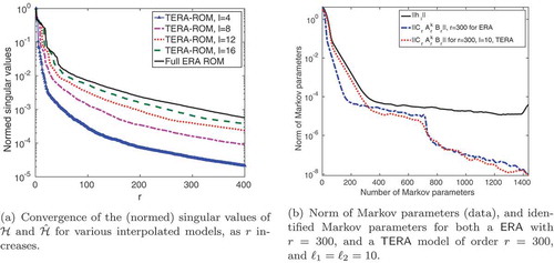
Figure 1. MSD model: The Markov parameters decay slowly in time (a); the singular values of the matrices ${\mathrm{\Theta }}_L$ and ${\mathrm{\Theta }}_R$ help guide the decision about the number of input/output interpolation directions needed (b).

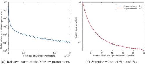
Figure 2. MSD model: The normalized singular values of the Hankel matrices $\mathcal{H}$ and $\hat{\mathcal{H}}$ are shown in decreasing order. With an increasing number of interpolation directions ${\mathrm{\ell }}_1={\mathrm{\ell }}_2$, the singular value decay curves approach the singular value decay of the full Hankel matrix $\mathcal{H}$.

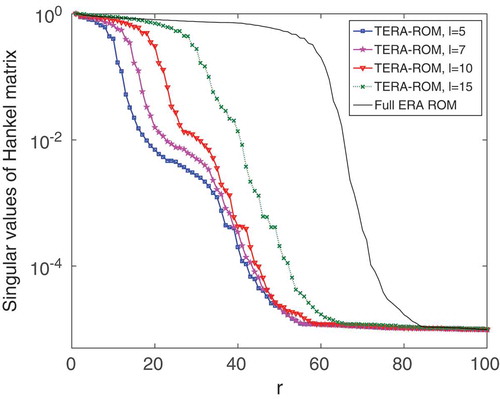
Figure 3. MSD model: Outputs of continuous-time simulations from the full model, and reduced models with $r=30$. In this case, TERA-ROM matches the output of the full order model better, whereas ERA shows strong deviations compared to the full order model.

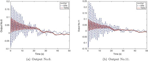
Figure 4. MSD model: Outputs of continuous-time simulations from the full model, and reduced models with $r=60$. At higher reduced order dimension, ERA performs better, and is visually indistinguishable from the full model.

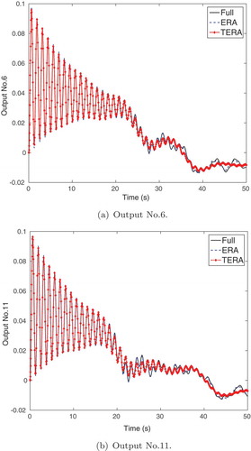
Figure 5. MSD model: Transfer function for ERA and TERA where ROMS have order $r=80$, and the TERA models were obtained by interpolating the data with a different number of directions. In plot (a), the original transfer function shows a peak around $\omega =2$. In both (a) and (b), ERA remains unchanged, and we show that TERA approaches the transfer function obtained from ERA as we increase the number of tangential directions.

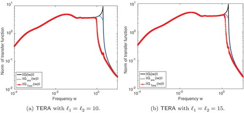
Figure 6. Rail model: Norm (relative) decay of the Markov parameters over time, $||h_i|{|}_F/||h_1|{|}_F$.

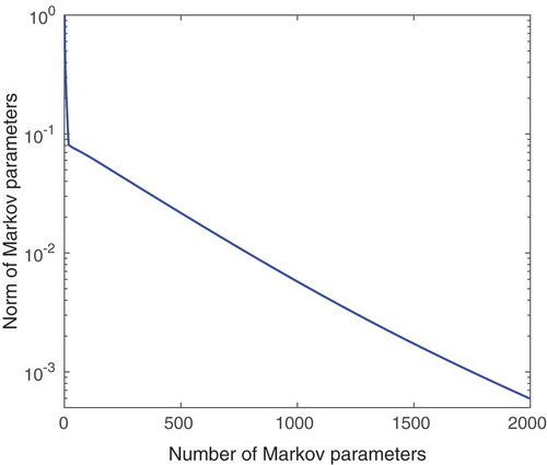
Figure 7. Rail model: The singular values of the matrices ${\mathrm{\Theta }}_L,{\mathrm{\Theta }}_R$ as well as of the Hankel matrix provide insight into truncation of input/output directions, as well as the ROM dimension $r$. In plot (b), for increasing numbers of tangential directions, the singular value decay approaches the behaviour of the ERA model, as expected.

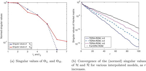
Figure 8. Rail model: Bode plots (transfer function) for full model, and the reduced-order models through ERA and TERA. As seen from (a), the transfer functions in the original scaling are visually identical. Thus, plot (b) shows the error of TERA and ERA with respect to the original transfer function.

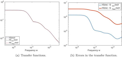
Figure 9. Rail model: The error bound of ERA (normalized) from (12) and TERA from (26) versus the actual errors.

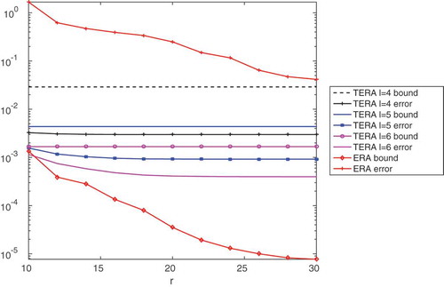
Figure 10. Rail model: The plot shows outputs of time domain simulations of the full and reduced-order models. In plot (a) and (b), all three models provide visually identical results, in plot (c), TERA shows a slight deviation for the first 20 s of simulation.

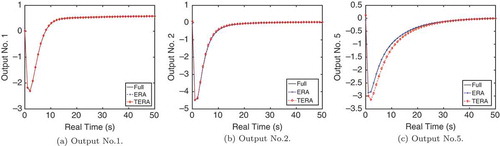
Figure 11. Rail model: Time domain simulations of the full and reduced-order models, where the TERA model was obtained by interpolation with random directions. The full model and the ERA model are visually indistinguishable on this scale.

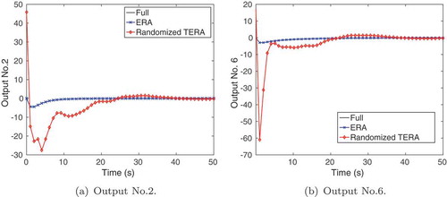
Figure 12. Indoor-air model: A high number of interpolation directions is needed to retain enough information from the sequence of Markov parameters. Especially plot (b) shows that decay of the singular values for ${\mathrm{\Theta }}_L,{\mathrm{\Theta }}_R$ with respect to ${\mathrm{\ell }}_1,{\mathrm{\ell }}_2$ is very slow.

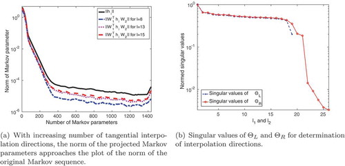
Figure 13. Indoor-air model: The TERA models slowly approach the ERA model as the number of interpolation directions ${\mathrm{\ell }}_1={\mathrm{\ell }}_2$ is increased, see plot (a). Part (b) shows that even the identified Markov parameters from a full ERA model do not match the original sequence well.