Determination of individual knee-extensor properties from leg extensions and parameter identification

Figures & data

Figure 1. Illustration of models A and B within the inclined leg press. (a) Shows the modelled leg and muscle–tendon complex within the leg press. (b) Points out the structural differences between model A and model B. Model A has no length dependencies and thus requires no CE length. Model B uses $l_{C{E}_{opt}}=0.09$ m [5,8] (reached at ${\alpha }_{opt}={120}^{\circ }$ [4]), and $l_{SEE,slack}=l_p$ (reached at the fully extended knee). (a) Geometrical relations (proportions are not in scale) of the leg within the leg press. The angles in the sketch are: γ the inclination of the leg press, α the knee-extension angle, β the angle between the force vector of the modelled muscle–tendon complex and the knee moment arm r, β′ the angle between r and the patellar tendon. The forces are: f_int the force of the muscle–tendon complex and F_ext the external force at the force plate. The lengths are: X the distance from the greater trochanter to the lateral malleolus, l_t the length of the thigh, l_s the length of the shank, l_MTC the length of the muscle–tendon complex, l_p the distance from the centre of the patella to the tibial tuberosity, ${\tilde{l}}_p$ the distance from the centre of the knee to the tibial tuberosity. (b) Schematic representation of the muscle–tendon complex f_int of models A and B. f_int of model A consists of a contractile element CE. Model B is an extension to model A adding a serial elastic element SEE and a force–length relation.

Figure 2. Time evolution of the activation dynamics at an isometric contraction. The activation dynamics represent the recruitment of muscle fibres until the maximum number of available fibres is reached. The initial activation $A_{pre}$ is constant and the additional force production starts at the onset $t_0$.

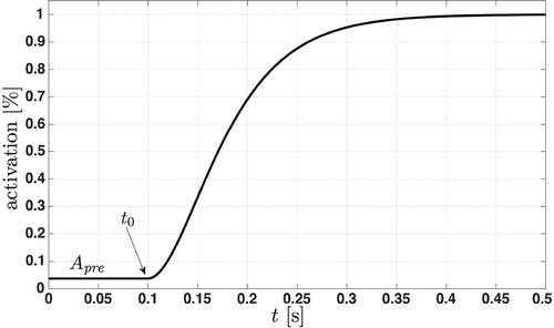
Figure 3. Examples of the SEE at dynamic (a) and isometric (b) contractions. (a) Force–time plot showing the differences between model outputs. External forces F_mod of model A, model B_k6e6n1 using a linear serial elastic element, and model B_k6e6n2.5 using a non-linear serial elastic element are shown. The subscript “k” and “n” are k_SEE,lin and n_SEE,nl, respectively. For each simulation, the conditions as well as the properties of the geometrical relations, of the contractile element, and of the activation dynamics are identical. (b) This force–elongation plot shows the force-dependent elongation of the non-linear serial elastic element from an isometric simulation (n_SEE,nl = 2.5, k_SEE,lin = 6 · 10⁶). The non-linear region is represented by the dotted line, whereas the solid line indicates the linear region. Due to the force–length relationship, the maximum isometric force f_iso = 18000 N is not reached. The thresholds at the transition from non-linear to linear are f_MTC,TH and ∆l_SEE,TH, respectively.

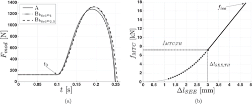
Figure 4. Parameter identification flow chart illustrating re-identification from simulated data sets (dotted grey arrows) and identification from measured data (solid black arrows). Double arrows mark comparisons.

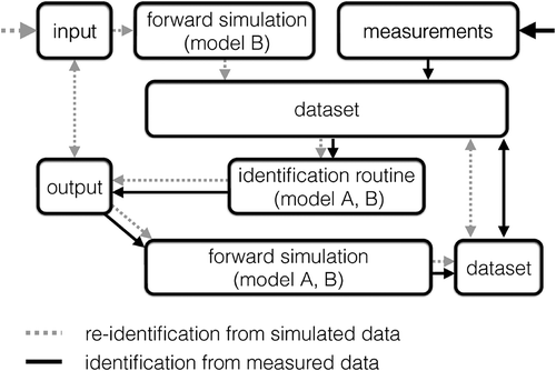
Figure 5. Force–time plot showing the identification process from measured data $F_{meas}$ (grey) using model ${\mathrm{B}}_{k_{\mathrm{i}\mathrm{d}}{n}_1}$. Data from dynamic measurements are offset to 0.3 and 0.7 s for better visibility. The connected diamonds represent the final stage of the identification $F_{opt}$ while the dashed line is the output $F_{sim}$ of the subsequent forward simulation.

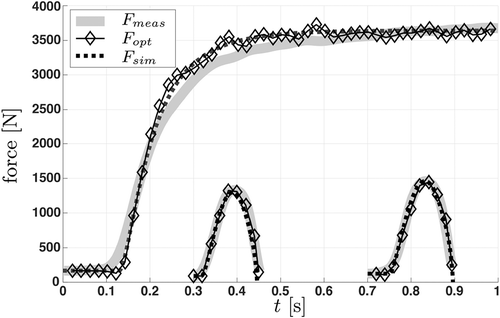
Table 1. Description of model B identification configurations. For enhanced readability the subscripts ‘k’ and ‘n’ represent $k_{SEE,lin}$ and $n_{SEE,nl}$, respectively. Subscripts ‘id’, ‘lit’ and ‘In’ are abbreviations for: parameter identified, parameter from literature and custom fixed input.

	U, $f_{iso}$, $v_{max}$, ${\eta }_{max}$, $t_{0,20,40,ISO}$	$k_{SEE,lin}$	$n_{SEE,nl}$	FL	dof
${\mathrm{B}}_{k_{\mathrm{I}\mathrm{n}}{n}_{\mathrm{I}\mathrm{n}}}$	Identified	Preset to In	Preset to In	On	7
${\mathrm{B}}_{k_{\mathrm{i}\mathrm{d}}{n}_{\mathrm{I}\mathrm{n}}}$	Identified	Identified	Preset to In	On	8
${\mathrm{B}}_{k_{\mathrm{i}\mathrm{d}}{n}_{\mathrm{i}\mathrm{d}}}$	Identified	Identified	Identified	On	9
${\mathrm{B}}_{k_{\mathrm{l}\mathrm{i}\mathrm{t}}{n}_1}$	Identified	Preset to lit	Preset to ‘1’	On	7
$B_{k_{\mathrm{l}\mathrm{i}\mathrm{t}}{n}_{2.5}}$	Identified	Preset to lit	Preset to ‘2.5’	On	7
${\mathrm{B}}_{k_{\mathrm{i}\mathrm{d}}{n}_1}$	Identified	Identified	Preset to ‘1’	On	8
${\mathrm{B}}_{k_{\mathrm{i}\mathrm{d}}{n}_{2.5}}$	Identified	Identified	Preset to ‘2.5’	On	8
${\mathrm{B}}_{k_{\mathrm{i}\mathrm{d}}{n}_1}^{\star }$	Identified	Identified	Preset to ‘1’	Off	8
${\mathrm{B}}_{k_{\mathrm{i}\mathrm{d}}{n}_{2.5}}^{\star }$	Identified	Identified	Preset to ‘2.5’	Off	8

Table 2. Re-identifying parameters from two sets of simulated data with model B${ }_{\mathrm{i}\mathrm{d}}$ configurations.

		$U\left(\frac{1}{\mathrm{s}}\right)$	$f_{iso}$ (N)	$p_{max}$ (W)	$v_{max}\left(\frac{\mathrm{m}}{\mathrm{s}}\right)$	$\frac{a}{f_{iso}}$	${\eta }_{max}$	$k_{SEE,lin}\left(\frac{\mathrm{N}}{\mathrm{m}}\right)$	$n_{SEE,nl}$
	In	20	18,000	1825	0.8	0.44	0.2	6,000,000	2.5
	Out	20	18,000.1	1825	0.8	0.44	0.2	.	.
${\mathrm{B}}_{k_{\mathrm{I}\mathrm{n}}{n}_{\mathrm{I}\mathrm{n}}}$	$\delta$$\cdot {10}^{-6}$	−105	5.56	11	−70	168.17	−145	.	.
	$c_v$	0.25	0.06	0.36	0.16	0.71	0.61	.	.
	Out	20	17,999.6	1825.2	0.8	0.44	0.2	6,006,963.66	.
${\mathrm{B}}_{k_{\mathrm{i}\mathrm{d}}{n}_{\mathrm{I}\mathrm{n}}}$	$\delta$$\cdot {10}^{-6}$	−55	−22.22	109.6	135	−6.82	5	1160.61	.
	$c_v$	0.05	0.02	0.11	0.09	0.14	0.12	0.55	.
	Out	20	18,000.1	1824.5	0.8	0.44	0.2	5,988,994.6	2.49
${\mathrm{B}}_{k_{\mathrm{i}\mathrm{d}}{n}_{\mathrm{i}\mathrm{d}}}$	$\delta$$\cdot {10}^{-6}$	190	4.14	−235.62	80	−713.6	610	−1834.23	−2273
	$c_v$	0.1	0.02	0.16	0.09	0.3	0.25	1.23	0.85
	In	20	18,000	1825	0.8	0.44	0.2	6,000,000	1
	Out	20	18,000.1	1824.9	0.8	0.44	0.2	.	.
${\mathrm{B}}_{k_{\mathrm{I}\mathrm{n}}{n}_{\mathrm{I}\mathrm{n}}}$	$\delta$$\cdot {10}^{-6}$	−70	5.56	−38.4	8.75	−113.6	95	.	.
	$c_v$	0.18	0.05	0.26	0.12	0.52	0.44	.	.
	Out	20	18,000	1825	0.8	0.44	0.2	6,000,118.8	.
$\underset{\_}{{\mathrm{B}}_{k_{\mathrm{i}\mathrm{d}}{n}_{\mathrm{I}\mathrm{n}}}}$	$\delta$$\cdot {10}^{-6}$	−1.6	−0.37	3.5	−1.04	8.42	−7.66	19.79	.
	$c_v$	0.17	0.03	0.19	0.07	0.4	0.34	2	.
	Out	20.2	18,010.3	1808.9	0.8	0.43	0.2	5,480,874.1	0.96
${\mathrm{B}}_{k_{\mathrm{i}\mathrm{d}}{n}_{\mathrm{i}\mathrm{d}}}$	$\delta$$\cdot {10}^{-6}$	8885	573	−8817	2541	−26,255	22,953	−86,521	−39,171
	$c_v$	0.09	0.01	0.2	0.13	0.35	0.29	0.79	1.07

Input parameters: In; identified parameters: Out; coefficient of variation: $c_v$; relative error: $\delta$. The underlined model is the best candidate to identify $k_{SEE,lin}$.

Table 3. Parameter average $\mu$ and standard deviation ($\sigma$) of identified parameters from model A and model B. The underlined model is the best candidate to identify $k_{SEE,lin}$.

		$U\left(\frac{1}{\mathrm{s}}\right)$	$f_{iso}$ (N)	$p_{max}$ (W)	$v_{max}\left(\frac{\mathrm{m}}{\mathrm{s}}\right)$	$\frac{a}{f_{iso}}$	${\eta }_{max}$	$k_{SEE,lin}\left(\frac{\mathrm{N}}{\mathrm{m}\mathrm{m}}\right)$	$r_a^{2}sim$
A	$\mu$	21.9	16,756	1640	0.95	0.3	0.27	.	0.99
	$\sigma$	(4.7)	(3602)	(297)	(0.1)	(0.08)	(0.04)	(.)	(0.009)
${\mathrm{B}}_{k_{\mathrm{l}\mathrm{i}\mathrm{t}}{n}_1}$	$\mu$	22.9	16,891	1543	0.95	0.27	0.3	.	0.99
	$\sigma$	(4.7)	(3667)	(267)	(0.1)	(0.08)	(0.05)	(.)	(0.009)
${\mathrm{B}}_{k_{\mathrm{l}\mathrm{i}\mathrm{t}}{n}_{2.5}}$	$\mu$	22.8	17,000	1504	0.89	0.29	0.29	.	0.99
	$\sigma$	(4.6)	(3733)	(255)	(0.1)	(0.08)	(0.05)	(.)	(0.008)
$\underset{\_}{{\mathrm{B}}_{k_{\mathrm{i}\mathrm{d}}{n}_1}}$	$\mu$	28	17,849	1253${ }_{†††}^{\ast \ast }$	0.95	0.18${ }_{†††}^{\ast \ast }$	0.38${ }_{†††}^{\ast \ast \ast }$	1777	0.99
	$\sigma$	(6.5)	(4229)	(211)	(0.1)	(0.08)	(0.07)	(324)	(0.008)
${\mathrm{B}}_{k_{\mathrm{i}\mathrm{d}}{n}_{2.5}}$	$\mu$	21.8	16,803	1640	0.94	0.31	0.27	73,370	0.99
	$\sigma$	(4.5)	(3626)	(302)	(0.1)	(0.09)	(0.05)	(46,650)	(0.009)
${\mathrm{B}}_{k_{\mathrm{i}\mathrm{d}}{n}_1}^{\star }$	$\mu$	29.6	16,914	1191	0.94	0.18	0.38	1701	0.99
	$\sigma$	(6.7)	(3685)	(202)	(0.1)	(0.06)	(0.06)	(292)	(0.009)
${\mathrm{B}}_{k_{\mathrm{i}\mathrm{d}}{n}_{2.5}}^{\star }$	$\mu$	22.2	16,760	1605	0.94	0.3	0.28	87,580	0.99
	$\sigma$	(4.5)	(3602)	(324)	(0.12)	(0.08)	(0.05)	(41,080)	(0.009)

**$p\le 0.01$, ${ }^{\ast \ast \ast }$ $p\le 0.001$, ${ }_{†††}$ $g^{\ast }\ge 0.8$.

Models B are compared to A, and models ${\mathrm{B}}_{k_{\mathrm{i}\mathrm{d}}}^{\star }$ are compared to ${\mathrm{B}}_{k_{\mathrm{i}\mathrm{d}}}.$

Table 4. Parameter coefficient of variation from model A and configurations of model B. Averaged values: $\mu$; standard deviations: ($\sigma$).

		U	$f_{iso}$	$p_{max}$	$v_{max}$	$\frac{a}{f_{iso}}$	${\eta }_{max}$	$k_{SEE,lin}$
A	$\mu$	0.09	0.007	0.19	0.1	0.3	0.21	.
	$\sigma$	(0.03)	(0.003)	(0.08)	0.04	(0.11)	(0.07)	(.)
${\mathrm{B}}_{k_{\mathrm{l}\mathrm{i}\mathrm{t}}{n}_1}$	$\mu$	0.14	0.009	0.27	0.15	0.42	0.29	.
	$\sigma$	(0.06)	(0.005)	(0.11)	(0.06)	(0.18)	(0.14)	(.)
${\mathrm{B}}_{k_{\mathrm{l}\mathrm{i}\mathrm{t}}{n}_{2.5}}$	$\mu$	0.1	0.006	0.2	0.11	0.31	0.2	.
	$\sigma$	(0.05)	(0.002)	(0.11)	(0.06)	(0.15)	(0.09)	(.)
$\underset{\_}{{\mathrm{B}}_{k_{\mathrm{i}\mathrm{d}}{n}_1}}$	$\mu$	0.2${ }_{†††}^{\ast }$	0.25${ }_{†††}^{\ast }$	0.31	0.19	0.39	0.21	0.3
	$\sigma$	(0.14)	(0.02)	(0.2)	(0.14)	(0.23)	(0.15)	(0.36)
${\mathrm{B}}_{k_{\mathrm{i}\mathrm{d}}{n}_{2.5}}$	$\mu$	0.16	0.017	0.29	0.19	0.43	0.31	20.6
	$\sigma$	(0.11)	(0.018)	(0.23)	(0.14)	(0.33)	(0.24)	(20.6)
${\mathrm{B}}_{k_{\mathrm{i}\mathrm{d}}{n}_1}^{\star }$	$\mu$	0.18	0.007${ }_{†††}^{\ast }$	0.25	0.15	0.33	0.18	0.22
	$\sigma$	(0.08)	(0.004)	(0.11)	(0.06)	(0.15)	(0.09)	(0.18)
${\mathrm{B}}_{k_{\mathrm{i}\mathrm{d}}{n}_{2.5}}^{\star }$	$\mu$	0.14	0.008	0.24	0.15	0.36	0.25	19
	$\sigma$	(0.06)	(0.005)	(0.09)	(0.06)	(0.14)	(0.1)	(13)

* $p\le 0.05$, ${ }^{\ast \ast }$ $p\le 0.01$, ${ }_{†††}$ $g^{\ast }\ge 0.8$.

Models B are compared to A, and models ${\mathrm{B}}_{\mathrm{i}\mathrm{d}}^{\star }$ are compared to B ${ }_{\mathrm{i}\mathrm{d}}.$

Table 5. Relative changes in the correlation matrix using measured data sets. The values represent the correlations of the identified parameters of model ${\mathrm{B}}_{k_{\mathrm{i}\mathrm{d}}{n}_1}$ relative to model A.

	U	$v_{max}$	$f_{iso}$	${\eta }_{max}$	$t_{0,20}$	$t_{0,40}$	$t_{0,ISO}$
U	$\cdot$	–	${1.6}_{††}^{\ast \ast \ast }$	${1.3}_{†††}^{\ast \ast \ast }$	${0.79}_{†††}^{\ast \ast \ast }$	${0.71}_{†††}^{\ast \ast \ast }$	${0.27}_{†††}^{\ast \ast \ast }$
$v_{max}$	–	$\cdot$	–	–	–	–	${0.6}_{†}^{\ast }$
$f_{iso}$	${1.6}_{†††}^{\ast \ast \ast }$	–	$\cdot$	${4.2}_{†}^{\ast \ast \ast }$	${0.65}_{††}^{\ast \ast \ast }$	–	${1.9}_{†††}^{\ast \ast \ast }$
${\eta }_{max}$	${1.3}_{†††}^{\ast \ast \ast }$	–	${4.2}_{†††}^{\ast \ast \ast }$	$\cdot$	${0.65}_{†††}^{\ast \ast \ast }$	${0.48}_{†††}^{\ast \ast \ast }$	${0.26}_{†††}^{\ast \ast \ast }$
$t_{0,20}$	${0.79}_{†††}^{\ast \ast \ast }$	–	${0.65}_{†††}^{\ast \ast \ast }$	${0.65}_{†††}^{\ast \ast \ast }$	$\cdot$	${0.94}_{†††}^{\ast \ast \ast }$	${0.58}_{†††}^{\ast \ast }$
$t_{0,40}$	${0.71}_{†††}^{\ast \ast \ast }$	–	–	${0.48}_{††}^{\ast \ast \ast }$	${0.94}_{†††}^{\ast \ast \ast }$	$\cdot$	${0.63}_{†††}^{\ast }$
$t_{0,ISO}$	${0.27}_{†††}^{\ast \ast \ast }$	${0.6}_{†††}^{\ast }$	${1.9}_{†††}^{\ast \ast \ast }$	${0.26}_{†††}^{\ast \ast \ast }$	${0.58}_{†††}^{\ast \ast }$	${0.63}_{†††}^{\ast }$	$\cdot$

${ }^{\ast }$ p ≤ 0.05, ${ }^{\ast \ast }$ $p\le 0.01$, ${ }^{\ast \ast \ast }$ $p\le 0.001$, ${ }_{†}$ $g^{\ast }<0.5$, ${ }_{††}$ $g^{\ast }<0.8$, ${ }_{†††}$ $g^{\ast }\ge 0.8$.

Figure 6. Boxplots of identified $a/f_{iso}$ from measured data sets and different models. Note that only models ${\mathrm{B}}_{k_{\mathrm{i}\mathrm{d}}{n}_1}$ and ${\mathrm{B}}_{k_{\mathrm{i}\mathrm{d}}{n}_1}^{\star }$ are significantly different from the others.

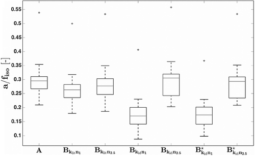
Table 6. Parameter range ($Pa{r}_{max}$ – $Pa{r}_{min}$ without outliers), mean parameter accuracies $\mu \left\{acc\right\}$ and $\mu \left\{ac{c}_{\mathrm{\%}}\right\}$ defined as $\mu \left\{acc\right\}$ normalized to the range (cf. Equation (29)).

		$U\left(\frac{1}{\mathrm{s}}\right)$	($f_{iso}$N)	($p_{max}$W)	$v_{max}\left(\frac{\mathrm{m}}{\mathrm{s}}\right)$	$\frac{a}{f_{iso}}$	${\eta }_{max}$	$k_{SEE,lin}\left(\frac{\mathrm{N}}{\mathrm{m}\mathrm{m}}\right)$
A	$Pa{r}_{max}$	29.7	22,781	2102	1.14	0.35	0.32	.
	$Pa{r}_{min}$	16.52	12,875	1045	0.81	0.21	0.24	.
	$\mu \left\{acc\right\}$	2	117	331	0.1	0.09	0.06	.
	$\mu \left\{ac{c}_{\mathrm{\%}}\right\}$	(15%)	(1.2%)	(30%)	(28%)	(62%)	(70%)	.
${\mathrm{B}}_{k_{\mathrm{i}\mathrm{d}}{n}_1}$	$Pa{r}_{max}$	40.54	24,085	1676	1.14	0.23	0.51	2271
	$Pa{r}_{min}$	20.64	13,295	921.2	0.81	0.09	0.32	1353
	$\mu \left\{acc\right\}$	5.6	4462	234	0.18	0.07	0.08	533
	$\mu \left\{ac{c}_{\mathrm{\%}}\right\}$	(28%)	(41%)	(31%)	(54%)	(50%)	(42%)	(58%)

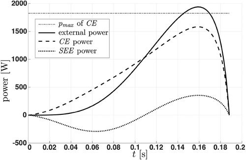
Figure 7. Power–time plot of a simulated leg extension. The horizontal line ($p_{max}$ of CE) indicates the maximum power of the contractile element. Initially, the serial elastic element (SEE, dotted line) stores energy and returns it towards the end of the movement. Thus, it is possible that the external power (solid line) exceeds the power of the contractile element (CE, dashed line). Note that due to the influences of the force–length relation and the activation function, the power of the contractile element does not reach its maximum value $p_{max}$.

M.G. Pandy, F.E. Zajac, E. Sim, and W.S. Levine, An optimal control model for maximum-height human jumping, J Biomech 23 (1990), pp. 1185–1198. doi:10.1016/0021-9290(90)90376-E

 PubMed Web of Science ®Google Scholar

A.J. Van Soest and M.F. Bobbert, The contribution of muscle properties in the control of explosive movements, Biol. Cybern 69 (1993), pp. 195–204. doi:10.1007/BF00198959

 PubMed Web of Science ®Google Scholar

M.G. Hoy, F.E. Zajac, and M.E. Gordon, A musculoskeletal model of the human lower extremity: The effect of muscle, tendon, and moment arm on the moment-angle relationship of musculotendon actuators at the hip, knee, and ankle, J. Biomech 23 (1990), pp. 157–169. doi:10.1016/0021-9290(90)90349-8

 PubMed Web of Science ®Google Scholar