Towards real-time fluid dynamics simulation: a data-driven NN-MPS method and its implementation

Figures & data

Figure 1. The arrangement of particles near the wall.

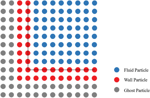
Figure 2. A description of a particle and its neighborhood.

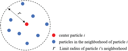
Figure 3. The velocity update scheme in the proposed NN-MPS method.

Figure 4. A description of the neural network. For each neuron in the hidden layer, the nonlinear activation function is the ReLU. Each of the first two hidden layers has eight neurons, and the last hidden layer has four neurons.

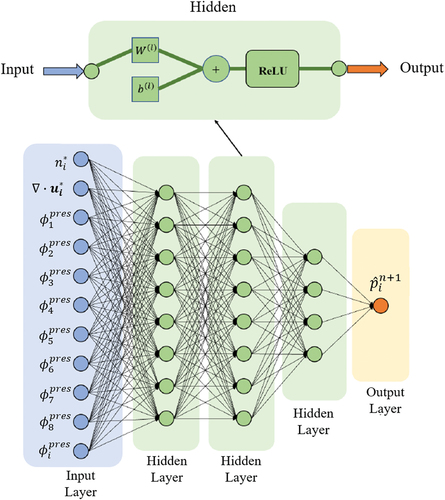
Figure 5. A Visualization of $W^l$ and $b^l$, $l=\left\{1,2,3\right\}$, in (2) after training. The vectors at the top are $b$ and the matrices at the bottom are $W$. From left to right: $1^{st}$ layer, $2^{nd}$ layer, $3^{rd}$ layer, $4^{th}$ layer.

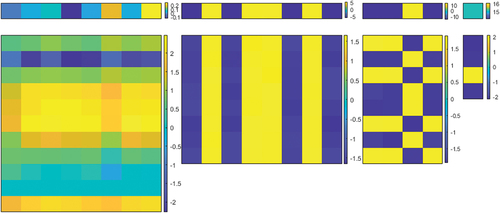
Figure 6. A visualization of the training set. From left to right: scene 1, scene 2, scene 3, scene 4.

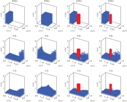
Table 1. Parameters of different scenes in the training set. The time step is set to 0.003 s and the simulation time of all scenes is 1.5 s (500 steps). The initial distance is set to 0.075. The size implies the number of particles, where $r$ is the radius, $h$ is the height, $l$ is the length and $w$ is the width.

Scene	Box size	Column size	Obstacle size	Obstacle position
1	$32\times 16\times 20$	$8\times 16\times 20$	$-$	$-$
2	$32\times 16\times 20$	$16\times 16\times 20$	$-$	$-$
3	$32\times 16\times 20$	$8\times 16\times 20$	$r=3,h=20$	$(1.4250,0.8250)$
4	$32\times 16\times 20$	$8\times 16\times 20$	$r=w=3,h=20$	$(1.4250,0.8250)$

Figure 7. A visualization of the dam collapse problem. Upper: NN-MPS. Lower: Original MPS. From left to right: $0.3s,0.6s,0.9s,1.2s,1.5s$.

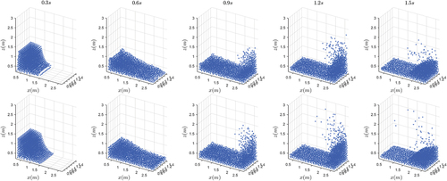
Table 2. The parameters setting for the dam collapse problem.

Parameters	Value
Initial distance for particles $l_0$	$0.075m$
Gravitational acceleration $g$	$9.81$$m^2/s$
Water kinematic viscosity $\nu$	$1\times {10}^{-6}$$m^2/s$
Coefficient of collision $e$	0.2
Time interval of each frame $\mathrm{\Delta }t$	0.003s
Tank size	$32l_0\times 16l_0\times 20l_0$
Column size	$8l_0\times 16l_0\times 18l_0$

Figure 8. A comparison of pressure distribution at $0.3s$, $0.9s$, and $1.5s$ (from left to right). Top row: NN-MPS; Bottom row: Original MPS.

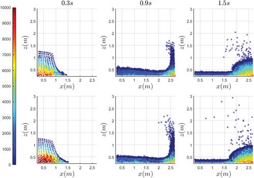
Figure 9. A comparison of the position of fluid front and pressure at bottom of the left wall.

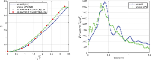
Figure 10. The pressure and the pressure gradient of flow field. Left: With one-cylinder obstacle. Right: With a two-cylinder obstacle. Upper: Pressure at bottom of the left wall. Lower: $z$ component of pressure gradient at bottom of the left wall.

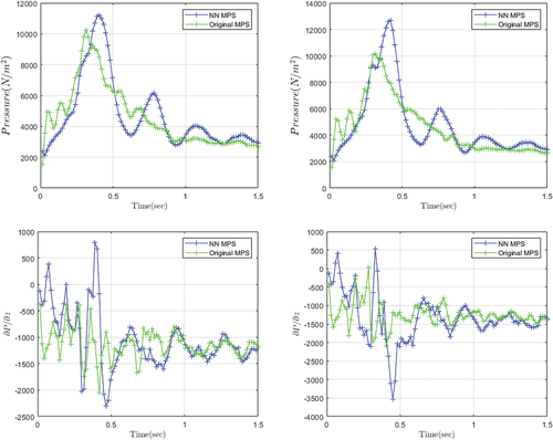
Figure 11. A comparison of two algorithms on the problem with a one-cylinder obstacle. Top row: NN-MPS. Bottom row: MPS.

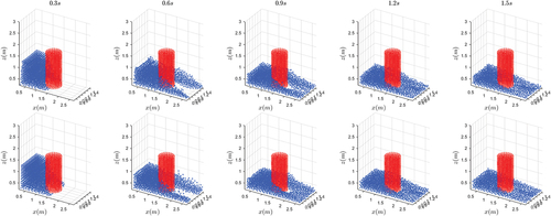
Figure 12. A comparison of two algorithms on the problem with a two-cylinder obstacle. Top row: NN-MPS. Bottom row: MPS.

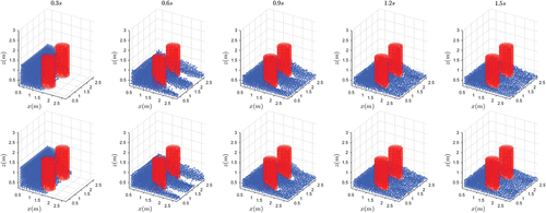
Table 3. The parameters setting for the dam collapse problem.

Case	Description	Box size	Total particle numbers	Pressure caculation using time
				MPS	NN-MPS(CPU)	NN-MPS(GPU)
1	Column collapse(1)	$32l_0\times 16l_0\times 16l_0$	13056	1.45s	0.42s	0.04s
2	Column collapse(2)	$64l_0\times 32l_0\times 32l_0$	54528	16.93s	3.55s	0.05s
3	Column collapse(3)	$96l_0\times 48l_0\times 48l_0$	136962	86.97s	9.92s	0.11s
4	One-cylinder obstacle	$40l_0\times 16l_0\times 16l_0$	15316	1.45s	0.42s	0.04s
5	Two-cylinder obstacle	$40l_0\times 32l_0\times 16l_0$	13056	1.45s	0.42s	0.04s

Figure 13. The ratio of pressure calculation time.

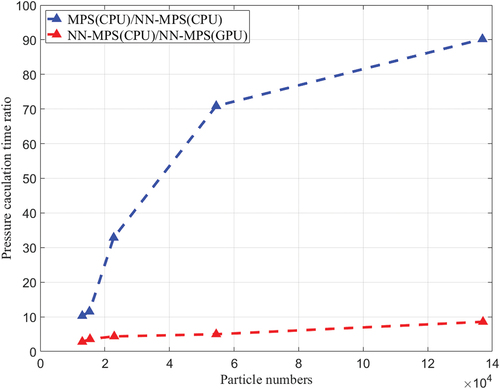
Figure 14. An illustration of the multi-precision strategy used on ascend 310.

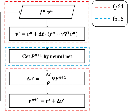
Figure 15. A description of dividing the domain into grids and distributing the grids to different processes.

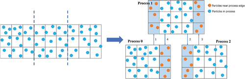
Figure 16. A visualization of three testing models.

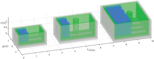
Table 4. The model sizes and speedup.

Index	Box size	Fluid particles	CPU	AI core	Speedup
1	$[30,20,14]\times 0.075$	1456	0.2932s	0.035s	8.37815
2	$[40,24,20]\times 0.075$	2048	0.2955s	0.036s	8.2077
3	$[40,48,20]\times 0.075$	10240	0.5882s	0.12052s	4.8805

Figure 17. Numerical results of the free-surface movement. (a) shows the definition of $X$ and $H$. (b), (c) and (d) respectively show the results of models with index number 1, 2 and 3.

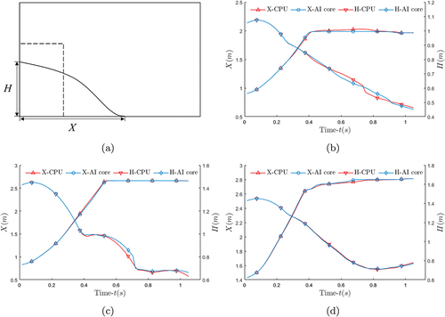
Figure 18. Pressure results at left corner. (a), (b) and (c) respectively show the results of models with index number 1, 2 and 3.

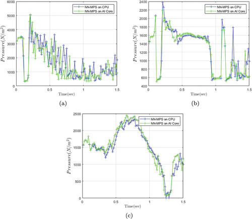
Figure 19. A comparison of two different devices on the problem with case 1. Top row: CPU. Bottom row: AI Core.

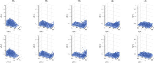
Figure 20. A comparison of two different devices on the problem with case 2. Top row: CPU. Bottom row: AI Core.

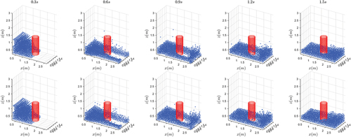
Figure 21. A comparison of two different devices on the problem with case 3. Top row: CPU. Bottom row: AI Core.

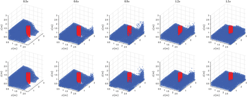
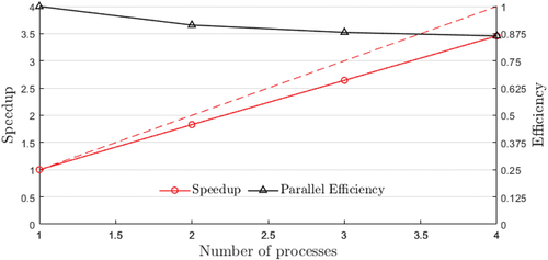
Figure 22. The parallel efficiency and speedup.