Figures & data
Figure 1. CT image as shown in the 3DSlicer interface (a), and segmented bronchi on the same slice as yellow label map (b).
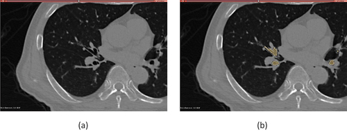
Figure 2. Kitaoka lung model generated for tracheobronchial tree in the left upper lobe (LUL) (a), Combining Kitaoka tree with CT resolved geometry (b), Location of Boolean Union highlighted in blue (c) and Hybrid lung model used in CFD analysis (d).
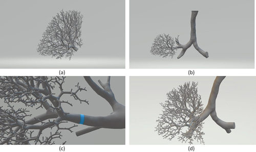
Table 1. Calculation of fractional lobar volume change using results reported by Yamada et al. [Citation33].
Figure 3. Cut-out view of airway showing discretization with mesh refinement near walls (a), and Results from mesh independence study: LR profile (b) and AP profile (c).
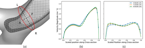
Figure 4. Comparison of Simulation Result with Experimental Data Showing LR profile (a), AP profile (b), Previous Numerical Data (c).
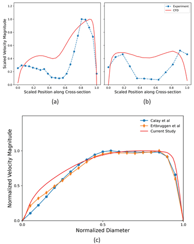
Figure 5. Pressure probe location on simplified pig airway geometry (a) and comparison between calculated pressure drop with experimental result (b).
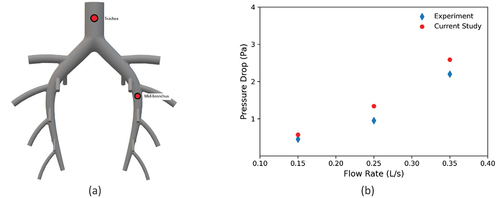
Figure 6. Contours of total pressure for flow rate of 30 l/min (a) and 15 l/min (b). Profiles in middle airway (first section) are on top and profiles in distal airways (second section) are at the bottom.
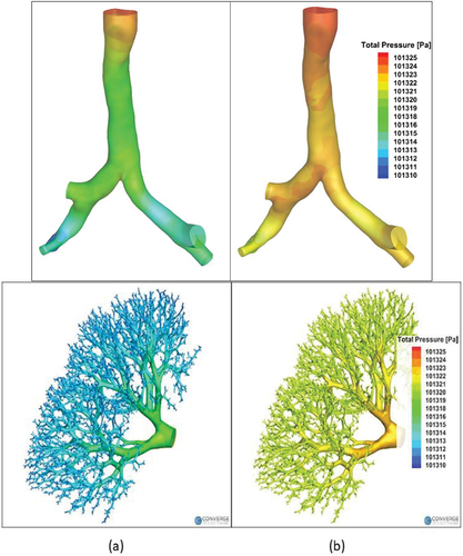
Figure 7. Velocity field in the 1st section for flow rate of 30 l/min and 15 l/minPlane Slice Showing Contours of Velocity Magnitude (a) Vector Contours of Secondary Velocity near inlet cross-section (b) and carinal section(c).
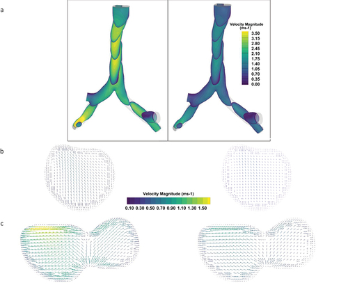
Figure 8. Contours of axial velocity magnitude in distal airways starting from generation 3 up to generation 21 for 30l/min and 15l/min.
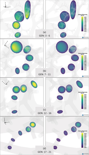
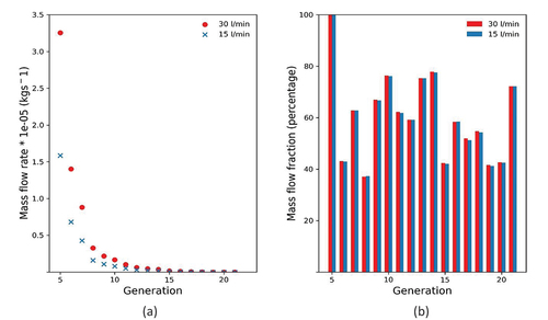
Figure 9. Mass flow rate in the distal generations (a) and mass flow fractions in terms of flow in parent branch (b) through the selected airway path.