The stabilizing effect of small prey immigration on competitive predator-prey dynamics

Figures & data

Table 1. List of symbols with their biological meaning.

symbol	The meaning
r	Inherent growth rate of prey
k	Carrying capacity of the system
u	Death rate of predator
$\mathit{\alpha }$	Accessibility parameter of prey by a predator
h	Handling and digestion rates of the predator
e	Efficiency of converting consumed prey into predator birth
$\frac{m}{x}$	Few prey immigrants

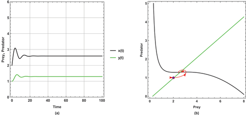
Figure 1. Prey predator dynamics of the system (1) when $(\mathit{m}=0)$: (a) time series (b) nullclines and phase portrait trajectories. Other parametric and initial values are: $\mathit{r}=1$, $\mathit{k}=6$, $\mathit{\alpha }=0.8$, $\mathit{u}=0.5$, $\mathit{e}=0.4$, $\mathit{x}(0)=2$, $\mathit{y}(0)=1$.

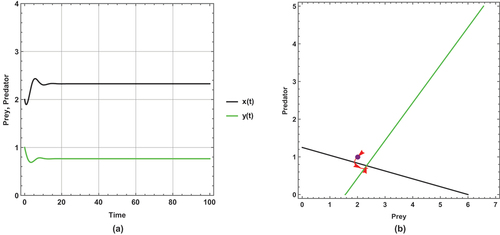
Figure 2. Prey predator dynamics of the system (1) when $(\mathit{m}=1.0)$: (a) time series (b) nullclines and phase portrait trajectories. Other parametric and initial values are: $\mathit{r}=1$, $\mathit{k}=6$, $\mathit{\alpha }=0.8$, $\mathit{u}=0.5$, $\mathit{e}=0.4$, $\mathit{x}(0)=2$, $\mathit{y}(0)=1$.

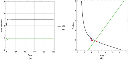
Figure 3. Prey predator dynamics of the system (1) when $(\mathit{m}=3.0)$: (a) time series (b) nullclines and phase portrait trajectories. Other parametric and initial values are: $\mathit{r}=1$, $\mathit{k}=6$, $\mathit{\alpha }=0.8$, $\mathit{u}=0.5$, $\mathit{e}=0.4$, $\mathit{x}(0)=2$, $\mathit{y}(0)=1$.

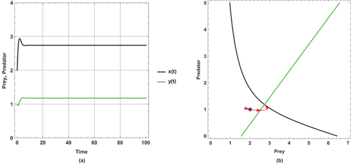
Figure 4. (a) Time series (b) nullclines and phase portrait trajectories of the first set of system (2) when $(\mathit{m}=0)$. Other parametric and initial values are: $\mathit{r}=1$, $\mathit{k}=6$, $\mathit{\alpha }=3.25$, $\mathit{h}=0.40$, $\mathit{u}=0.5$, $\mathit{e}=0.4$, $\mathit{x}(0)=2$, $\mathit{y}(0)=1$.

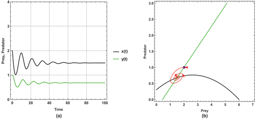
Figure 5. (a) Time series (b) nullclines and phase portrait trajectories of the first set of system (2) when $(\mathit{m}=0.5)$. Other parametric and initial values are: $\mathit{r}=1$, $\mathit{k}=6$, $\mathit{\alpha }=3.25$, $\mathit{h}=0.40$, $\mathit{u}=0.5$, $\mathit{e}=0.4$, $\mathit{x}(0)=2$, $\mathit{y}(0)=1$.

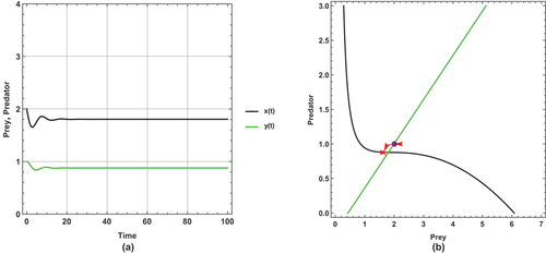
Figure 6. (a) Time series (b) nullclines and phase portrait trajectories of the first set of system (2) when $(\mathit{m}=2.0)$. Other parametric and initial values are: $\mathit{r}=1$, $\mathit{k}=6$, $\mathit{\alpha }=3.25$, $\mathit{h}=0.40$, $\mathit{u}=0.5$, $\mathit{e}=0.4$, $\mathit{x}(0)=2$, $\mathit{y}(0)=1$.

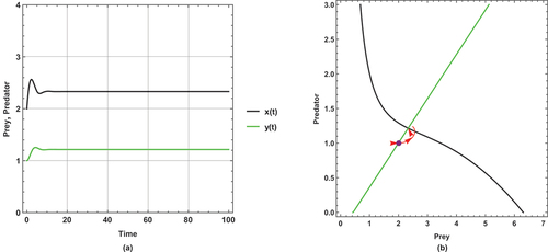
Figure 7. (a) Time series (b) nullclines and phase portrait trajectories of the second set of system (2) when $(\mathit{m}=0)$. Other parametric and initial values are: $\mathit{r}=1$, $\mathit{k}=8$, $\mathit{\alpha }=7.00$, $\mathit{h}=0.50$, $\mathit{u}=0.45$, $\mathit{e}=0.5$, $\mathit{x}(0)=2$, $\mathit{y}(0)=1$.

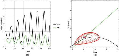
Figure 8. (a) Time series (b) nullclines and phase portrait trajectories of the second set of system (2) when $(\mathit{m}=0.1)$. Other parametric and initial values are: $\mathit{r}=1$, $\mathit{k}=8$, $\mathit{\alpha }=7.00$, $\mathit{h}=0.50$, $\mathit{u}=0.45$, $\mathit{e}=0.5$, $\mathit{x}(0)=2$, $\mathit{y}(0)=1$.

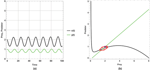
Figure 9. (a) Time series (b) nullclines and phase portrait trajectories of the second set of system (2) when $(\mathit{m}=1.5)$. Other parametric and initial values are: $\mathit{r}=1$, $\mathit{k}=8$, $\mathit{\alpha }=7.00$, $\mathit{h}=0.50$, $\mathit{u}=0.45$, $\mathit{e}=0.5$, $\mathit{x}(0)=2$, $\mathit{y}(0)=1$.