It’s also about timing! When do pedestrians want to receive navigation instructions

Figures & data

Table 1. Actions taken based on the in-situ check of landmarks generated by the algorithm described by Rousell and Zipf (2017)

action	share of total amount of turning points (133)
suggested landmark used	36.8%
no landmark suggested	23.3%
changed due to potential ambiguity	16.5%
changed due to poor salience	12.0%
changed due to further reasons (e.g., non-existent POI or visibility value issues, see Rousell and Zipf (2017) for a detailed account)	11.4%

Figure 1. Example of potential ambiguity. At the illustrated turning point (yellow circle), participants would have to make a left turn. The algorithm described by Rousell and Zipf (2017) suggests to use the POI which is tagged with amenity:bank and named Erste Bank (green circle). Based on this, the route instruction would be (translated to English): Turn left at Erste Bank. However, this would have been ambiguous (see the red arrow) given the local spatial layout [source of background image: Filipe et. al (2020)].

Figure 2. Example of overestimated salience. The algorithm by Rousell and Zipf (2017) picks the beauty salon (red circle) as the most suitable landmark. However, this landmark cannot be recognized easily when approaching the turning point as can be derived from the picture on the left (for the specific spatial layout see the map on the right). The mall called Lugner City (highlighted in green) is clearly more salient and, hence, the algorithm’s choice was overruled by the experimenter [left: image by creator istefanos retrieved from Mapillary on Feb 26th, 2021, licensed under CC BY 4.0 and cropped); source of background image on the right: Filipe et. al (2020)].

Table

General structure	Imperative to turn	landmark	direction of turn
Example in German	Biegen Sie bei	der Apotheke	links ab.

Figure 3. A: A sample participant in full equipment. B: GNSS receiver (PPM 10-xx38). C: During the experiment, participants requested navigation instructions using a custom-built clicker-device (circled in red) which triggers an LED light located in the backpack informing the experimenter about the request.

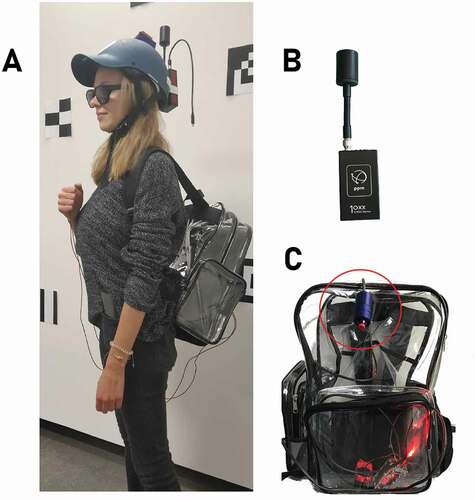
Figure 4. Segmentation process. Two possible situations: A (default case): The segment starts at the last turning point denoted as 3. The first intersection after the click position is denoted as 4 and the segment ends at this intersection. B: A route segment covering the distance from the starting point to intersection 2. It is reasonable to assume that the participant has not perceived intersection 1 as a decision point because the instruction is requested after it had been passed background image: Story 2013].

Table 2. Description of influential variables according to our model results. Categories: P: participant, R: route, T: trial, E: environment. Sources: OQ: online questionnaire that was completed by participants, UA: Urban Atlas, OSM: OpenStreetMap

Category	Variable	Description	Type	Unit	Source
P	age_gt_40	age greater than 40	dichotomous	N/A	OQ
	BFI_o_low	result of subscale openness of the BFI-10 scale; norm data threshold: < 3.41 (Rammstedt et al., 2012, p. 28)	dichotomous	N/A	OQ
	BFI_e_low	result of subscale extraversion of the BFI-10 scale; norm data threshold: < 3.47 (Rammstedt et al., 2012, p. 28)	dichotomous	N/A	OQ
	sum_ego	sum score of subfactor global/egocentric of the FRS questionnaire; this subscale reflects SOD according to Münzer et al. (2016)	7-point likert scale	N/A	OQ
R	lngSegm	segment length > $120m$	metric	meter	OSM
		Threshold based on lower and upper quartile of the segment length
T	familiar/ unfamiliar	participantis familiar/unfamiliar with a route and area it is located in	dichotomous	N/A	OQ
E	LC_*	landcover share of 50 m buffer around route segment; 1 = 12100; 2 = 11100 + 11210; 3 = 11220 + 11230; 12100, 11100, 11210, 11220, 11230 landcover codes of Urban Atlas (European Comission, 2012)	metric	%	UA

Table 3. Summary statistics of the observations used for model estimation. (d): denotes a dichotomous variable; for these variables column mean represents the proportion in the sample, SD: standard deviation, Min: minimum value, Max: maximum value, distance norm.: normalized distance; all other variable names are explained in Table 2

Variable	Mean	SD	Min	Max
distance norm.	0.498	0.329	0.007	1.000
lngSegm (d)	0.137	–	–	–
age_gt_40 (d)	0.075	–	–	–
LC_1	0.130	0.180	0	1
LC_2	0.424	0.286	0.000	0.90
LC_3	0.091	0.216	0.000	0.868
familiar (d)	0.419	–	–	–
unfamiliar (d)	0.581	–	–	–
sum_ego	51.17	9.88	16	68
BFI_e_low (d)	0.568	–	–	–
BFI_o_low (d)	0.424	–	–	–

Table 4. Normalized timing of instructions based on the AFT model. The variables are explained in Table 2

Variable	$\beta$	Robust SD error
age_gt_40	0.706***	0.143
LC_1	−0.587**	0.208
LC_2	−0.528***	0.151
LC_3	−0.490*	0.253
lngSegm	0.307***	0.170
sum_ego	−0.007***	0.002
lngSegm:unfamiliar	−0.628**	0.233
unfamiliar:BFI_e_low	0.240*	0.113
unfamiliar:BFI_o_low	−0.407**	0.125
Log(scale)	−0.366***	0.078
Scale $\sigma$	0.694
Observations	241
$L_p$: LogLikelihood	−40.5
$L_0$: LogLikelihood (intercept only)	−59.1
Nagelkerke $R^2$	0.143
AIC	101.09
$p$ value: + $p<0.1$; * $p<0.05$; ** $p<0.01$; *** $p<0.001$

Figure 5. Predicted median survival values based on the estimated AFT model compared against the observed ones.

Figure 6. Empirical survival rates for two given subsets of observations ($BFI\mathrm{\_}o\mathrm{\_}low=1$; $BFI\mathrm{\_}e\mathrm{\_}low=1$; $lngSegm=1$; $age\mathrm{\_}gt\mathrm{\_}40=0$; left: familiar, right: unfamiliar segments), compared against the mean predicted ones. Dotted lines represent the 95% CI.

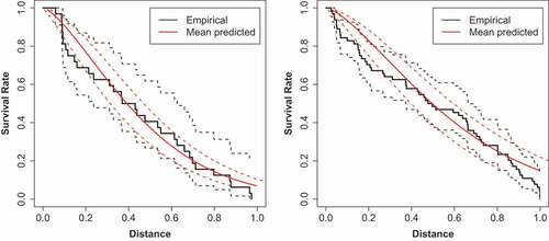
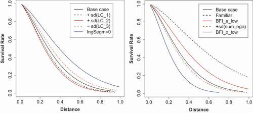
Figure 7. Variation of survival rate predictions due to explanatory variables modifications (continuous variables = $\pm$1 standard deviation ($SD$), dummy variables =$\pm$1) compared to a base case scenario (BFI_o_low = 0, lngSegm = 1, age_gt_40 = 0, BFI_e_low = 0, unfamiliar = 1). Variable names are explained in Table 2.

Rousell, A., & Zipf, A. (2017). Towards a landmark-based pedestrian navigation service using OSM data. ISPRS International Journal of Geo-Information, 6(3), 64. doi:10.3390/ijgi6030064

 Web of Science ®Google Scholar

Zimmer, H. D., Münzer, S., & Baus, J. (2010). From Resource-Adaptive Navigation Assistance to Augmented Cognition. In M. W. Crocker & J. Siekmann (Eds.), Resource-Adaptive Cognitive Processes (pp. 35–53). Berlin, Heidelberg: Springer. doi: 10.1007/978-3-540-89408-7_3

 Google Scholar

Therneau, T. (2014). A package for survival analysis in S. R Package Version, 2.37-4.

 Google Scholar

Rammstedt, B., Kemper, C. J., Klein, M. C., Beierlein, C., & Kovaleva, A. (2012). Eine kurze Skala zur Messung der fünf Dimensionen der Persönlichkeit. GESIS-Working Papers, 22(2), 1–32.

 Google Scholar

Münzer, S., Fehringer, B. C., & Kühl, T. (2016). Validation of a 3-factor structure of spatial strategies and relations to possession and usage of navigational aids. Journal of Environmental Psychology, 47, 66–78. doi:10.1016/j.jenvp.2016.04.017

 Web of Science ®Google Scholar

Comission, E. (2012). Mapping Guide for a European Urban Atlas — Copernicus. urban-atlas-mapping-guide, 30, 2020). Retrieved from https://land.copernicus.eu/user-corner/technical-library/

 Google Scholar