3,961
Views
25
CrossRef citations to date
0
Altmetric
Articles

A Critical-Realist View of Housing Quality within the Post-Communist EU States: Progressing towards a Middle-Range Explanation

ORCID Icon & ORCID Icon

Figures & data

Figure 1. A critical-realist approach to housing quality.

Figure 1. A critical-realist approach to housing quality.

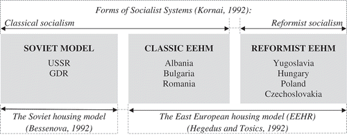
Figure 2. Theorizing communist housing systems.

Figure 2. Theorizing communist housing systems.

Table 1. New housing provision during communist period in selected countries (rounded %).

Table 2. Country values (grouped by former housing models/geographical regions).

Table 3. ANOVA test for cluster means with ranking scores for housing quality.

Table 4. Nuancing housing quality across four clusters (ANOVA test and ranking scores).

Figure 3. Market dynamics. Source: Authors’ compilation from HYPOSTAT (Citation2005, 2007, 2011, 2013, 2015, 2016) for all except Eurostat’s (Citation2016) mobility rates available at https://appsso.eurostat.ec.europa.eu/nui/show.do?data-set=ilc_hcmp05&lang=en.
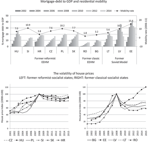
Figure 3. Market dynamics. Source: Authors’ compilation from HYPOSTAT (Citation2005, 2007, 2011, 2013, 2015, 2016) for all except Eurostat’s (Citation2016) mobility rates available at https://appsso.eurostat.ec.europa.eu/nui/show.do?data-set=ilc_hcmp05&lang=en.

Box 1. Our choice of indicators.

Figure 4. Clustering patterns (HCA on 19 variables). Source: SPSS software output. Notes: The visual clue is the length of the horizontal interval between two merging steps. The solution of three clusters is thus obvious. The three clusters remain stable upon the elimination of variable Q2 (see Figure A1 in the online annex) and/or the inclusion of five additional macro-indicators (i.e. GDP/capita in 1995; post-communist built stock; % homeoweners in total population; 2007–2012 residential mobility rates; % change in household numbers, see Figure A2 in the online annex).
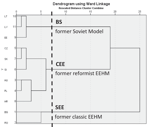
Figure 4. Clustering patterns (HCA on 19 variables). Source: SPSS software output. Notes: The visual clue is the length of the horizontal interval between two merging steps. The solution of three clusters is thus obvious. The three clusters remain stable upon the elimination of variable Q2 (see Figure A1 in the online annex) and/or the inclusion of five additional macro-indicators (i.e. GDP/capita in 1995; post-communist built stock; % homeoweners in total population; 2007–2012 residential mobility rates; % change in household numbers, see Figure A2 in the online annex).

Figure 5. Deconstructing clustering patterns by macro- and micro-indicators. Source: SPSS software output. Note: The three cluster solution (left side) and four cluster solution (right side) remain stable upon the elimination of variable Q2 and/or the inclusion of additional macro-indicators (i.e. GDP/capita in 1995; post-communist built stock; % homeoweners in total population; 2007–2012 residential mobility rates; % change in household numbers, see Figure A1 and A2 in the online annex).
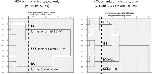
Figure 5. Deconstructing clustering patterns by macro- and micro-indicators. Source: SPSS software output. Note: The three cluster solution (left side) and four cluster solution (right side) remain stable upon the elimination of variable Q2 and/or the inclusion of additional macro-indicators (i.e. GDP/capita in 1995; post-communist built stock; % homeoweners in total population; 2007–2012 residential mobility rates; % change in household numbers, see Figure A1 and A2 in the online annex).
Supplemental material

Supplemental_material.docx

Download MS Word (279.7 KB)