An improved algorithm for dynamic nearest-neighbour models

Figures & data

Figure 1. Different networks, the nodes N of which are the stops of the national railway operator SJ in Sweden. (a) Network representation of the original network, (b) the Mocnik model for the nodes $N$ and $\rho =2$, and (c) a Gilbert model (Gilbert 1959) for the nodes $N$ and probability ${10}^{-3}$. The parameters are chosen such that similarities and dissimilarities visually stand out.

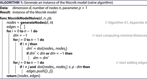
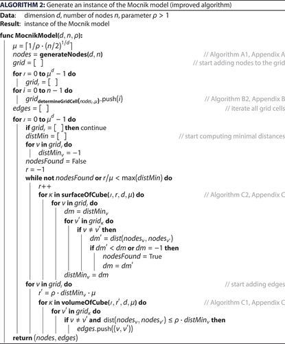
Table 1. Average-case time complexity of the algorithms discussed in this article. Algorithm 1 is the naïve and Algorithm 2 the improved algorithm for generating a Mocnik model. As Algorithms A1–C2 are of supplementary nature (they are used by Algorithms 1 and 2) they are discussed in the appendix. The complexity refers to the dimension $d$, the number of nodes $n$, the parameter $\rho$ of the Mocnik model, and, in case of Algorithms C1 and C2, to the radius r used in the algorithm. In Algorithm 2, the typical radius $\tilde{r}$ is a constant.

Algorithm	Complexity	Complexity (d and $\mathit{\rho }$ const.)
Algorithm 1	$O(d\cdot n^2+d\cdot (2/\sqrt{\pi }{)}^d\cdot \mathrm{\Gamma }(d/2+1)\cdot n)$	$O(n^2)$
Algorithm 2	$O(d\cdot (2/\sqrt{\pi }{)}^d\cdot \mathrm{\Gamma }(d/2+1)\cdot n+d\cdot {\rho }^d\cdot (2\tilde{r}{)}^d\cdot n)$	$O(n)$
Algorithm A1	$O(d\cdot (2/\sqrt{\pi }{)}^d\cdot \mathrm{\Gamma }(d/2+1)\cdot n)$	$O(n)$
Algorithm B1a	$O(d)$	$O(1)$
Algorithm B1b	$O(d)$	$O(1)$
Algorithm B2	$O(d)$	$O(1)$
Algorithm C1	$O(d\cdot (2r{)}^d)$	$O(r^d)$
Algorithm C2	$O(d^2\cdot (2r{)}^{d-1})$	$O(r^{d-1})$

Table 2. Algorithms related to the index and the spatial grid. The algorithms refer to the dimension $d$ of the space as well as to the number of grid cells per dimension $\mu$.

Algorithm	Symbol	Output
Algorithm B1a	toID$(c,\mu )$	ID ι of the grid cell with integer coordinates $c$
Algorithm B1b	fromID$(\iota ,d,\mu )$	integer coordinates $c$ of the grid cell with ID $\iota$
Algorithm B2	determineGridCell$(\nu ,\mu )$	ID of the grid cell containing the pair of coordinates $\nu$
Algorithm C1	volumeOfCube$(\iota ,r,d,\mu )$	IDs of the grid cells forming the hypercube centred at $\iota$ and with a radius of $⌈r⌉$
Algorithm C2	surfaceOfCube$(\iota ,r,d,\mu )$	IDs of the grid cells forming the surface of the hypercube centred at $\iota$ and with a radius of $r$

Figure 2. Spatial grid for indexing nodes. The grid consists of ${\mu }^d$ cells, where $d$ is the dimension and $\mu$ an integer. Each cell is of edge length $2/\mu$.

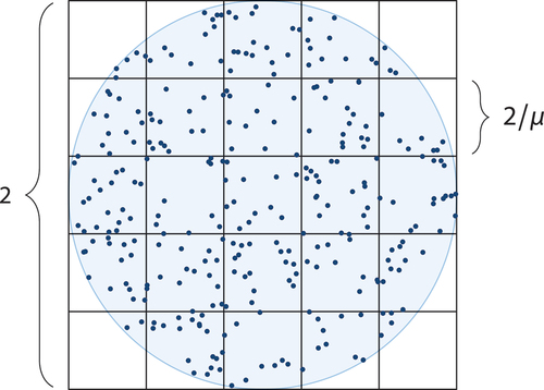
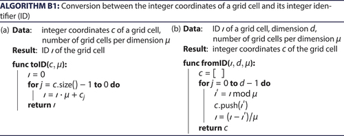
Figure 3. Identifiers (IDs) for the spatial grid. The function toID translates from integer coordinates to IDs, while the function fromID translates into the opposite direction.

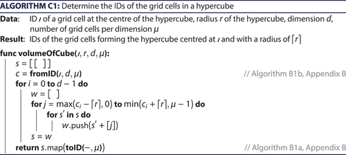
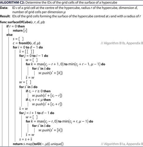
Figure 4. Volumes and surfaces in the spatial grid. (a) Volumes in the spatial grid, marked in blue, form hypercubes of adjacent cells. They are determined by their centre cell, here marked by a cross, and their radius. The volume at radius $r$ is contained in the volume of radius $r+1$. (b) The surface at radius $r$ is the volume at radius $r$ with the volume at radius $r-1$ removed.

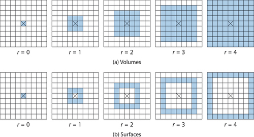
Table 3. Running times of the naïve and the improved algorithm. The running times refer to the generation of a Mocnik model with parameter $\rho =1.6$. All times are given in seconds.

	d = 2			d = 3
Number of nodes	Naïve	Improved	Improved parallel	Naïve	Improved	Improved parallel
5.0·10^2	2.16·10^−^3	5.19·10^−^3	3.02·10^−^3	2.60·10^−^3	1.05·10^−^2	6.14·10^−^3
1.0·10^3	6.58·10^−^3	9.57·10^−^3	6.24·10^−^3	8.90·10^−^3	2.52·10^−^2	1.39·10^−^2
2.5·10^3	4.11·10^−^2	2.70·10^−^2	1.54·10^−^2	4.47·10^−^2	6.25·10^−^2	3.59·10^−^2
5.0·10^3	1.47·10^−^1	5.31·10^−^2	2.86·10^−^2	1.72·10^−^1	1.24·10^−^1	7.12·10^−^2
7.5·10^3	3.11·10^−^1	8.34·10^−^2	4.23·10^−^2	3.73·10^−^1	1.88·10^−^1	1.08·10^−^1
1.0·10^4	5.76·10^−^1	1.00·10^−^1	5.82·10^−^2	6.59·10^−^1	2.56·10^−^1	1.44·10^−^1
2.5·10^4	3.37·10^0	2.49·10^−^1	1.45·10^−^1	3.91·10^0	6.53·10^−^1	3.57·10^−^1
5.0·10^4	1.31·10^1	5.02·10^−^1	2.89·10^−^1	1.47·10^1	1.29·10^0	7.18·10^−^1
7.5·10^4	2.83·10^1	7.36·10^−^1	4.39·10^−^1	3.31·10^1	1.91·10^0	1.14·10^0
1.0·10^5	5.05·10^1	9.79·10^−^1	6.21·10^−^1	6.01·10^1	2.56·10^0	1.52·10^0
2.5·10^5	3.46·10^2	2.50·10^0	1.56·10^0	3.99·10^2	6.53·10^0	3.84·10^0
5.0·10^5	1.36·10^3	5.13·10^0	3.21·10^0	1.62·10^3	1.32·10^1	7.94·10^0
7.5·10^5	3.07·10^3	7.88·10^0	4.93·10^0	3.58·10^3	1.98·10^1	1.19·10^1
1.0·10^6	5.26·10^3	1.05·10^1	6.62·10^0	6.19·10^3	2.80·10^1	1.58·10^1

Figure 5. Running times of the naïve and the improved algorithm for generating a Mocnik model ($\mathit{\rho }\mathbf{=}\mathbf{1}\mathbf{.6}$). (compare Table 3)

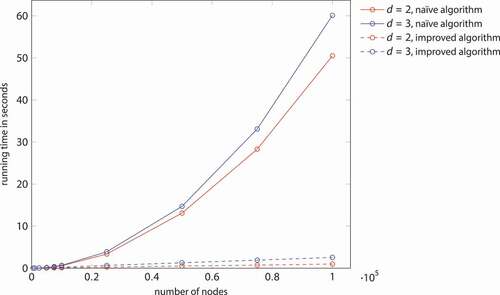
Figure 6. Running times of the improved algorithm for generating a Mocnik model ($\mathit{\rho }\mathbf{=}\mathbf{1}\mathbf{.6}$), both with and without parallel execution. (compare Table 3)

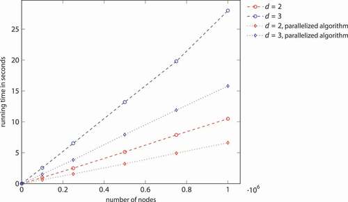
Table D1. Running times of the naïve and the improved algorithm, depending on the dimension of the embedding space. The running times refer the generation of a Mocnik model with 10,000 nodes and parameter $\rho =1.6$. All times are given in seconds.

Dimension	Naïve	Improved	Improved parallel
1	5.13·10^−1	4.15·10^−2	2.55·10^−2
2	5.28·10^−1	9.47·10^−2	5.56·10^−2
3	6.13·10^−1	2.50·10^−1	1.37·10^−1
4	7.04·10^−1	6.70·10^−1	3.62·10^−1
5	8.61·10^−1	1.76·10^0	9.90·10^−1
6	1.08·10^0	3.50·10^0	1.87·10^0
7	1.30·10^0	7.64·10^0	3.89·10^0
8	1.55·10^0	4.43·10^0	2.57·10^0
9	2.30·10^0	7.80·10^0	4.71·10^0
10	3.98·10^0	1.48·10^0	8.77·10^0

Table D2. Running times of the naïve and the improved algorithm, depending on the parameter $\mathit{\rho }$. The running times refer the generation of a Mocnik model with 10,000 nodes. All times are given in seconds.

	d = 2			d = 3
$\mathit{\rho }$	Naïve	Improved	Improved parallel	Naïve	Improved	Improved parallel
1.1	5.47·10^−1	1.14·10^−1	5.92·10^−2	6.15·10^−1	2.61·10^−1	1.35·10^−1
1.3	5.39·10^−1	9.88·10^−2	5.41·10^−2	6.26·10^−1	2.49·10^−1	1.39·10^−1
1.5	5.35·10^−1	9.95·10^−2	5.54·10^−2	6.45·10^−1	2.44·10^−1	1.39·10^−1
1.7	5.78·10^−1	9.62·10^−2	5.91·10^−2	6.73·10^−1	2.60·10^−1	1.43·10^−1
1.9	5.41·10^−1	1.05·10^−1	5.90·10^−2	6.49·10^−1	2.64·10^−1	1.50·10^−1
2.1	5.60·10^−1	9.95·10^−2	5.87·10^−2	6.46·10^−1	2.76·10^−1	1.52·10^−1
2.3	5.69·10^−1	1.01·10^−1	5.92·10^−2	6.95·10^−1	2.87·10^−1	1.62·10^−1
2.5	5.64·10^−1	1.03·10^−1	6.14·10^−2	6.69·10^−1	3.19·10^−1	1.77·10^−1
2.7	5.52·10^−1	1.03·10^−1	6.12·10^−2	6.57·10^−1	3.15·10^−1	1.79·10^−1
2.9	5.47·10^−1	1.09·10^−1	6.36·10^−2	6.49·10^−1	3.65·10^−1	2.04·10^−1
3.1	5.49·10^−1	1.09·10^−1	6.75·10^−2	6.46·10^−1	3.69·10^−1	2.08·10^−1
3.3	5.55·10^−1	1.12·10^−1	6.76·10^−2	6.44·10^−1	3.70·10^−1	2.12·10^−1
3.5	5.59·10^−1	1.14·10^−1	6.83·10^−2	6.78·10^−1	4.51·10^−1	2.59·10^−1
3.7	5.62·10^−1	1.16·10^−1	7.25·10^−2	6.79·10^−1	4.50·10^−1	2.58·10^−1
3.9	5.65·10^−1	1.19·10^−1	7.36·10^−2	6.69·10^−1	4.55·10^−1	2.64·10^−1
4.1	5.63·10^−1	1.23·10^−1	7.50·10^−2	6.65·10^−1	4.65·10^−1	2.69·10^−1
4.3	5.64·10^−1	1.32·10^−1	7.85·10^−2	6.64·10^−1	6.30·10^−1	3.51·10^−1
4.5	5.52·10^−1	1.35·10^−1	8.09·10^−2	6.65·10^−1	6.41·10^−1	3.58·10^−1
4.7	5.60·10^−1	1.35·10^−1	8.26·10^−2	6.83·10^−1	6.38·10^−1	3.66·10^−1
4.9	5.75·10^−1	1.39·10^−1	8.74·10^−2	6.97·10^−1	6.58·10^−1	3.63·10^−1
5.1	5.55·10^−1	1.48·10^−1	9.10·10^−2	7.14·10^−1	6.57·10^−1	3.67·10^−1
5.3	5.90·10^−1	1.48·10^−1	9.02·10^−2	6.86·10^−1	6.73·10^−1	3.76·10^−1
5.5	5.88·10^−1	1.54·10^−1	9.49·10^−2	7.13·10^−1	6.66·10^−1	3.80·10^−1
5.7	5.78·10^−1	1.55·10^−1	9.52·10^−2	7.36·10^−1	9.51·10^−1	5.81·10^−1
5.9	5.74·10^−1	1.66·10^−1	1.01·10^−1	7.16·10^−1	9.50·10^−1	5.77·10^−1
6.1	6.07·10^−1	1.66·10^−1	1.03·10^−1	7.38·10^−1	9.86·10^−1	5.85·10^−1
6.3	5.69·10^−1	1.68·10^−1	1.03·10^−1	7.67·10^−1	9.75·10^−1	6.06·10^−1
6.5	5.86·10^−1	1.79·10^−1	1.09·10^−1	7.53·10^−1	9.78·10^−1	6.12·10^−1
6.7	5.84·10^−1	1.87·10^−1	1.11·10^−1	7.63·10^−1	9.84·10^−1	6.23·10^−1
6.9	5.81·10^−1	1.79·10^−1	1.13·10^−1	7.69·10^−1	1.01·10^0	6.35·10^−1
7.1	5.80·10^−1	1.95·10^−1	1.19·10^−1	7.93·10^−1	1.00·10^0	6.31·10^−1
7.3	5.80·10^−1	2.03·10^−1	1.21·10^−1	7.88·10^−1	1.03·10^0	6.55·10^−1
7.5	6.26·10^−1	1.96·10^−1	1.20·10^−1	7.93·10^−1	1.04·10^0	6.64·10^−1
7.7	5.95·10^−1	2.02·10^−1	1.22·10^−1	7.93·10^−1	1.06·10^0	6.74·10^−1
7.9	5.90·10^−1	2.17·10^−1	1.32·10^−1	8.11·10^−1	1.08·10^0	6.73·10^−1
8.1	5.89·10^−1	2.28·10^−1	1.32·10^−1	8.26·10^−1	1.12·10^0	6.99·10^−1
8.3	6.01·10^−1	2.20·10^−1	1.37·10^−1	8.44·10^−1	1.13·10^0	7.09·10^−1
8.5	6.05·10^−1	2.24·10^−1	1.35·10^−1	8.61·10^−1	1.14·10^0	7.43·10^−1
8.7	6.00·10^−1	2.25·10^−1	1.39·10^−1	8.52·10^−1	1.54·10^0	9.12·10^−1
8.9	6.05·10^−1	2.57·10^−1	1.56·10^−1	8.91·10^−1	1.6·10^0	9.19·10^−1
9.1	6.10·10^−1	2.58·10^−1	1.60·10^−1	9.07·10^−1	1.58·10^0	9.33·10^−1
9.3	6.06·10^−1	2.60·10^−1	1.55·10^−1	9.18·10^−1	1.59·10^0	9.52·10^−1
9.5	6.00·10^−1	2.59·10^−1	1.55·10^−1	9.43·10^−1	1.62·10^0	9.39·10^−1
9.7	6.02·10^−1	2.63·10^−1	1.61·10^−1	9.39·10^−1	1.65·10^0	1.00·10^0
9.9	6.03·10^−1	2.67·10^−1	1.62·10^−1	9.47·10^−1	1.69·10^0	1.00·10^0
10.1	6.07·10^−1	2.69·10^−1	1.62·10^−1	9.84·10^−1	1.69·10^0	1.01·10^0

Figure D1. Running times of the naïve and the improved algorithm, depending on the dimension of the embedding space. The running times refer the generation of a Mocnik model with 10,000 nodes and parameter ρ = 1.6. (compare Table D1)

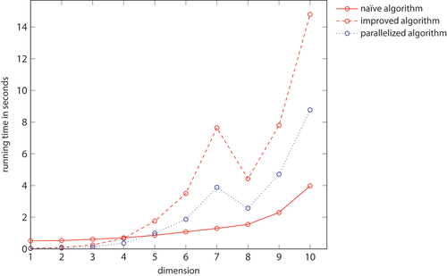
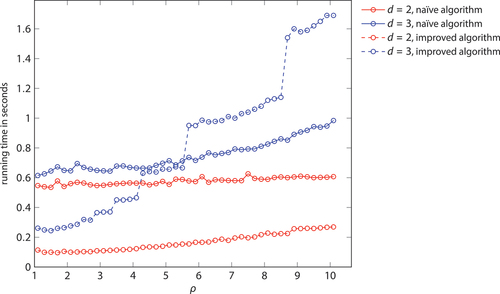
Figure D2. Running times of the naïve and the improved algorithm, depending on the parameter $\mathit{\rho }$. The running times refer the generation of a Mocnik model with 10,000 nodes. (compare Table D2)

Gilbert, E.N., 1959. Random graphs. Annals of Mathematical Statistics, 30 (4), 1141–1144. doi:10.1214/aoms/1177706098

 Google Scholar

Data availability statement

The algorithm has been implemented as part of NetworKit (Staudt et al. 2016), an open-source toolkit for large-scale network analysis. It is available on https://networkit.github.io.