Predicting the master curves of bituminous mastics with micromechanical modelling

Figures & data

Figure 1. The representative volume element used for the model with $\varphi =$ 30%, loaded uniaxially.

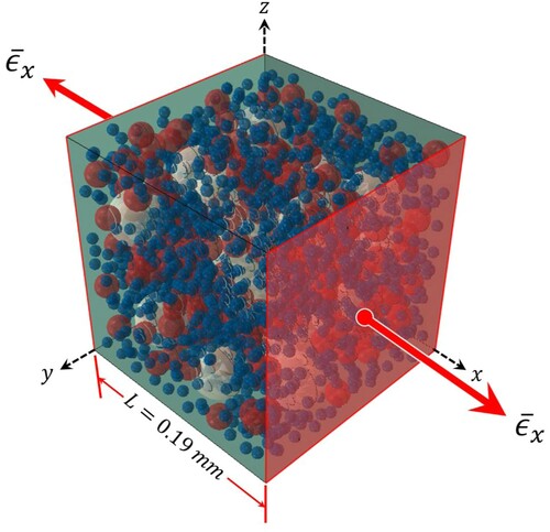
Figure 2. The response surface for the calculated complex modulus as a function of radial frequency and volume fraction.

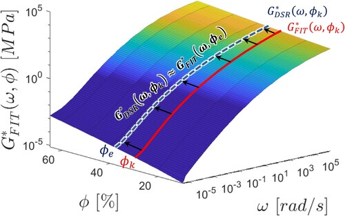
Figure 3. Master curves built for bitumen and mastics showing the complex modulus and the phase angle at a reference temperature $T_{ref}={20}^{\circ }\text{C}$.

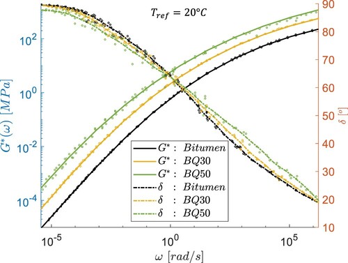
Table 1. Williams–Landel–Ferry constants.

Material	$C_1$	$C_2$
Bitumen	19.82	160.28
BQ30	19.54	150.12
BQ50	20.43	146.02

Figure 4. The size distribution of the quartz filler as well as the simplified size distributions used in the model, $d$ denotes the particle diameter.

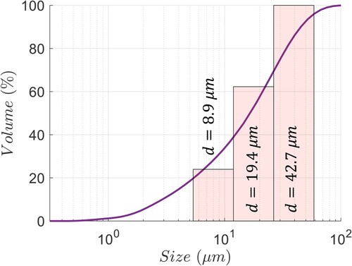
Figure 5. The calibrated model $G^{\ast }(\omega )$ compared to model before calibration and the experimental values for (a) ϕ = 30%, (b) ϕ = 50%, at reference temperature $T_{ref}={20}^{\circ }\text{C}$.

Figure 6. ${\nu }^{\ast }(\omega )$ for the bitumen and calculated ${\nu }^{\ast }(\omega )$ for the mastics obtained from FE simulations at a reference temperature $T_{ref}={20}^{\circ }\text{C}$.

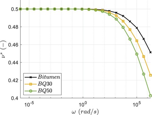
Figure 7. Equality plots for the measured DSR results as compared to the calibrated modelling results for (a) BQ30 and (b) BQ50.

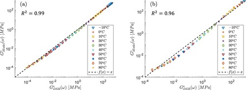
Figure 8. Comparison of the stiffness ratio obtained using the developed model, the generalised self-consistent scheme (GSCS), and the GSCS with limit values for (a) ϕ = 30%, (b) ϕ = 50%, at a reference temperature$T_{ref}={20}^{\circ }\text{C}$.

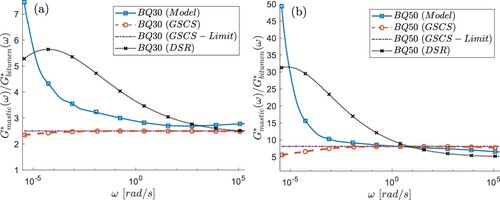
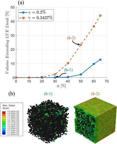
Figure 9. The maximum shear strain distribution within the micromechanical model at $z=L/2$ for applied effective shear strains 0.2% and 0.34% and for three filler volume fractions, $\varphi =$ 10%, 30% and 50% at reference temperature $T_{ref}=5^{\circ }\text{C}$ and $\omega =10\text{ rad/s}$.

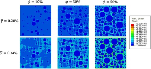
Figure 10. (a) Volume exceeding the linear-viscoelastic limit for two applied shear strains and (b) the corresponding element representation of said volume at reference temperature $T_{ref}=5^{\circ }\text{C}$.