On the role of pressure in elasto-inertial turbulence

Figures & data

Figure 1. Skin friction coefficient C_f as a function of the Reynolds number Re_H for two Weissenberg numbers, Wi_H = 4 (

) and Wi_H = 30 (

). Lines indicate correlations for laminar (· · · · · · · ·, C_f = 12/Re_H) and turbulent (– – – –, C_f = 0.073Re^{− 1/4}_H [11]) Newtonian channel flow, and for MDR (——, C_f = 0.42Re^{− 0.55}_H [12]); Newtonian solutions are also included (). Unlike for Newtonian flows, the skin friction of viscoelastic flows at sufficiently high Weissenberg number departs from the laminar correlation at subcritical Reynolds number and then smoothly transitions to the MDR asymptote.

Figure 2. Contour of the normalised polymer extension C_ii/L on selected planes and instantaneous isosurface of the second invariant Q_A of the velocity gradient tensor in the lower half of the channel for the subcritical case Re_H = 1000 and Wi_H = 4; Q_A = 0.1 (red) and Q_A = −0.1 (cyan). Trains of mostly spanwise cylindrical Q_A structures of alternating sign form around thin sheets of large polymer extension.

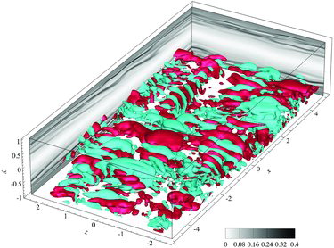
Table 1. Parameters used for the three viscoelastic and the Newtonian cases considered here. For all simulations, the FENE-P model is used with the maximum polymer extension parameter L = 200 and β = 0.9.

ReH^a	Reh^b	h^+^c	WiH^d	Wih^e	Wi^+^f	DM [%]^g	Colour^h
1000	500	40	4	8	24	+7
6000	3000	130	4	8	96	−56
6000	3000	120	30	60	720	−61
6000	3000	190	–	–	–	0

^aReynolds number based on the bulk velocity U_b and the total channel height H.

^bReynolds number based on the bulk velocity U_b and the channel half-height h (for comparison with previous publications).

^cChannel half-height h normalised by the friction velocity and the viscosity ν.

^dWeissenberg number based on the solution relaxation time λ and the integral time scale H/U_b.

^eWeissenberg number based on the solution relaxation time λ and the integral time scale h/U_b (for comparison with previous publications).

^fWeissenberg number based on the solution relaxation time λ and the wall-shear rate of the corresponding Newtonian case.

^g Drag modification (reduction or increase) measured as the relative change of the skin friction coefficient with the comparable Newtonian flow friction coefficient (laminar or turbulent).

^h Colour scheme used throughout the paper for each specific case.

Figure 3. Pressure rms as a function of y⁺. (a) Total pressure for the Newtonian case at Re_H = 6000 (

), and the viscoelastic cases Re_H = 1000, Wi_H = 4 (

); Re_H = 6000, Wi_H = 4 (HDR,

); and Re_H = 6000, Wi_H = 30 (MDR,

). (b)–(d) Pressure contributions for selected cases: p′_r ( — · — ); p′_s (· · · · · · · ·); p′_p ( – – – – ); p′_rs = p′_r + p′_s ( ——— ); p′_rsp = p′_r + p′_s + p′_p (

).

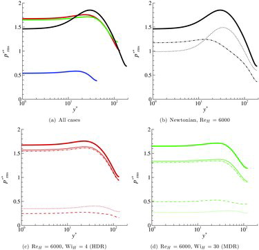
Figure 4. (a) Ratio of the polymeric p′_p to the inertial p′_rs pressure rms as a function of y⁺. (b) Ratio of the slow p′_s to the inertial p′_rs pressure rms as a function of y⁺. Same colour labels as in Figure 3.

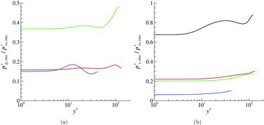
Figure 5. (a) and (b) Streamwise production terms ( – – – – ) and ( ——— ) as a function of y⁺. The polymer contribution is positive, indicating a transfer of energy from the polymers to the turbulence. (c) Wall-normal and spanwise production terms ( · · · · · · · · ) and ( — · — ) as a function of y⁺. In this case, energy is transferred from the turbulence to the polymers, but the levels are much lower than in the streamwise direction. Same colour labels as in Figure 3.

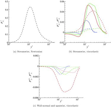
Figure 6. Streamwise pressure–strain component Φ⁺_xx as a function of y⁺ obtained from the different pressure contributions: p′_r ( — · — ); p′_s ( · · · · · · · · ); p′_p ( – – – – ); p′_rs = p′_r + p′_s (———); p′_rsp = p′_r + p′_s + p′_p (

). Same colour labels as in Figure 3. Φ_xx is negative in most of the domain indicating an energy transfer away from the streamwise component.

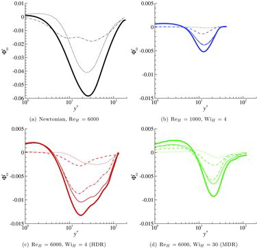
Figure 7. Wall-normal pressure–strain component Φ⁺_yy as a function of y⁺ obtained from different pressure contributions. Same line style as in Figure 6 and same colour labels as in Figure 3. Φ_yy is positive in most of the domain indicating an energy transfer to the wall-normal component.

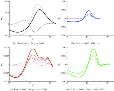
Figure 8. Spanwise pressure–strain component Φ⁺_zz as a function of y⁺ obtained from the different pressure contributions. Same line style as in Figure 6 and same colour labels as in Figure 3. Φ_zz is positive everywhere indicating an energy transfer to the spanwise component.

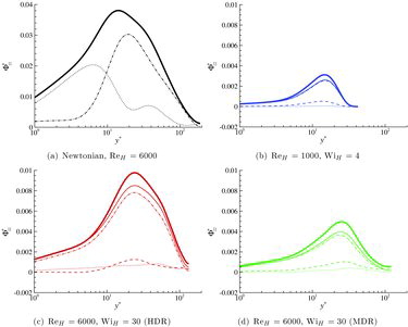
Figure 9. Production terms ( – – – – ) and ( ——— ) of Reynolds shear stress as a function of y⁺. Same colour labels as in Figure 3. Both terms cancel each other in the viscoelastic cases, explaining the very low levels of Reynolds shear stress observed.

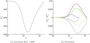
Figure 10. Pressure–strain component Π⁺_xy as a function of y⁺ obtained from the different pressure contributions: p′_r ( — - — ); p′_s (· · · · · · · ·); p′_p ( – – – – ); p′_rs = p′_r + p′_s ( ——— ); p′_rsp = p′_r + p′_s + p′_p (

). Same colour labels as in Figure 3.

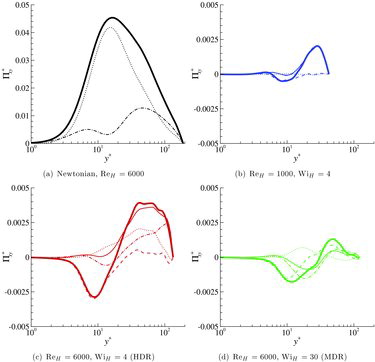
Figure 11. Instantaneous contour of the polymer stress component T_xx and isolines of Q_A (dash lines represent negative values) in an plane for Re_H = 1000 and Wi_H = 4. The flow is from left to right and the dashed box represents the region plotted in the next two figures.

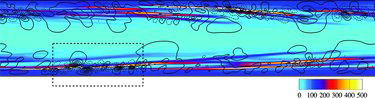
Figure 12. Instantaneous contour of the polymeric pressure contribution p_p and isolines of Q_A (dash lines represent negative values) in an plane for Re_H = 1000 and Wi_H = 4. The region plotted corresponds to the dashed box in Figure 11. A clear correlation between p_p and Q_A is visible.

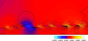
Figure 13. Instantaneous contour of the inertial pressure contribution p_rs and isolines of Q_A (dash lines represent negative values) in an plane for Re_H = 1000 and Wi_H = 4. The region plotted corresponds to the dashed box in Figure 11. Unlike the previous figure, no clear correlation between p_rs and Q_A is visible.

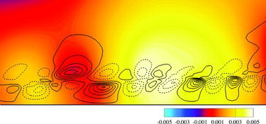
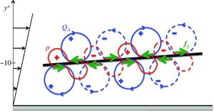
Figure 14. Schematics of the typical structures observed around thin sheets of large polymer extension (black line) in the near-wall region: second invariant of the velocity gradient tensor Q_A (blue), pressure p (red) and polymer body force (green). Dotted lines indicate a negative value.

R.D. Dean, Reynolds number dependence of skin friction and other bulk flow variables in two-dimensional rectangular duct flow, J. Fluids Eng. 100 (1978), pp. 215–222.

 Web of Science ®Google Scholar

P.S. Virk, E.W. Merrill, H.S. Mickley, K.A. Smith, and E.L. Mollo-Christensen, The Toms phenomenon: Turbulent pipe flow of dilute polymer solutions, J. Fluid Mech. 30 (1967), pp. 305–328.

 Web of Science ®Google Scholar