Figures & data
Figure 1. (a) Mass fraction of CO2, computed with CHEM1D, as a function of the x-coordinate, (b) Mass fraction of CH4 as a function of the non-scaled progress variable, i.e. .
Figure 2. (a) Source term of CO2, computed with CHEM1D, as a function of the x-coordinate in physical space, (b) source term of CO2 as a function of the scaled progress variable c obtained from the 1D FGM-manifold generated for the premixed laminar flame computed in (a). Additional examples obtained from the FGM database are (c) the temperature and (d) the density of the mixture.
Figure 3. 3D view of the computational domain showing the imposed mean profiles. For the inflow streamwise velocity profile, Ψ0 = U0 and Ψ1 = U1. For the scalar progress variable, Ψ1 = 0 denotes the unburned cold mixture while Ψ0 = 1 the outer hot co-flow burned products. The full domain size is 3D × 3D × 6D. The dashed lines denote the transition region of width D = 2.4 mm.
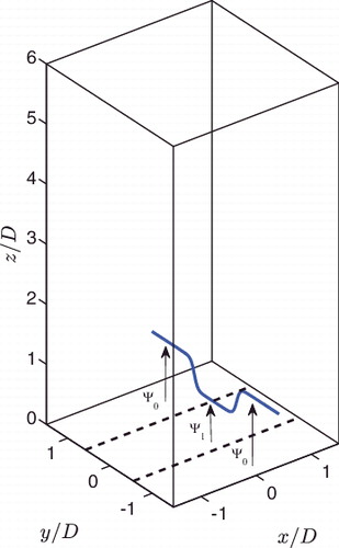
Figure 4. Spanwise autocorrelation functions of the streamwise fluctuations, Rxx, versus the spatial separation in the x-direction. The autocorrelation functions were obtained from a snapshot of the DNS field, collected after 25 flow through-times, and computed over the x-direction at constant y and z. Lines correspond to the results of Rxx obtained at y = 0.5D and z = z0, with z0 = 0.5D (dashed-dotted line), z0 = D (dashed line) and z0 = 1.5D (solid line). D represents the width of the inflow region, D=2.4 mm, associated with the cold low-speed stream.
Figure 5. Top view of the inflow plane showing 2D contours and vectors of the streamwise velocity component, wB, of the upstream modulation imposed at the inflow. The associated large-scale periodic flow is focused in the region of size L × D in the x- and y-direction. (left) the imposed pattern at K = 4π/L and (right) at K = 2π/L, respectively. The dashed lines represent the edges of the inflow plane region to which these coherent structures are concentrated.
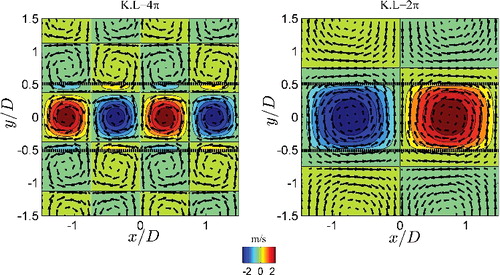
Figure 6. Unmodulated flame results: (a) Averaged flame front contours for the scalar c* and (b) Mean magnitude of the progress variable gradient ⟨|∇c|⟩, at different resolutions. Lines correspond to the following grids: 32 × 32 × 64 (dashed line), 64 × 64 × 128 (dashed-dotted line), and 128 × 128 × 256 (solid line).
Figure 7. (a) Total enstrophy ⟨Ω⟩xyz and (b) global averaged dissipation rate, ⟨ϵ⟩xyz, as a function of the spatial mode, KL/π. In this figure, both properties are normalised by the value of the reference unmodulated case, i.e. ⟨Ω0⟩xyz and ⟨ϵ0⟩xyz.
Figure 8. 3D snapshots of the flame front after 5 flow-through times coloured with vorticity in the z-direction, . Results for modulation wave-numbers from top left to bottom right: K = 24π/L, K = 6π/L, K = 4π/L, and K = 2π/L. The flame front corresponds to the surface of maximum heat release rate, i.e., c* = 0.56.
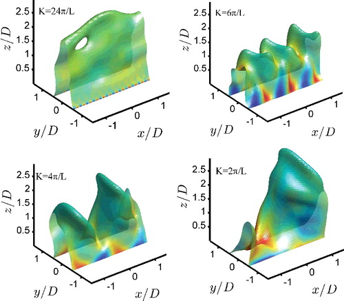
Figure 9. (Top) Results of the conditioned pdf of the magnitude of the scaled progress variable gradient versus the progress variable. The mean scalar gradient obtained for the one-dimensional premixed flamelet is also shown (solid line with ○ symbols), (bottom) variance of the mean scalar gradient, ⟨|∇c|2⟩ − ⟨|∇c|⟩2, as a function of c. In both figures, lines correspond to the following cases: unmodulated (dashed-dotted line), K = 24π/L (dotted line), 6π/L (dashed line), and 2π/L (solid line).
Figure 10. (Top) Results of the averaged global surface wrinkling ⟨W⟩ and (bottom) the averaged flame height ⟨H⟩ as a function of the modulation mode KL/π. The results of ⟨W⟩ are normalised by the global wrinkling obtained for the unmodulated reference case, W0, while the response quantity ⟨H⟩ is normalised by the width D.