Controlling Rayleigh–Bénard convection via reinforcement learning

Figures & data

Figure 1. Schematics of linear (a) and Reinforcement Learning (b) control methods applied to a Rayleigh–Bénard  system and aiming at reducing convective effects (i.e. the Nusselt number). The system consists of a domain with height, H, aspect ratio, $\mathrm{\Gamma }=1$, no-slip boundary conditions, constant temperature $T_C$ on the top boundary, adiabatic side boundaries and a controllable bottom boundary where the imposed temperature $T_B(x,t)$ can vary in space and time (according to the control protocol) while keeping a constant average $⟨T_B(x,t){⟩}_x=T_H$. Because the average temperature of the bottom plate is constant, the Rayleigh number is well defined and constant over time. The control protocol of the linear controller (a) works by calculating the distance measure $E(x,t)$ from the ideal state (cf. Equation 10(10) ${\hat{T}}_B(x,t)=\mathcal{R}({\tilde{T}}_B(x,t))=-\mathcal{R}((k_P-k_D{\mathrm{\partial }}_t)E(x,t))$(10) –11(11) $E(x,t)=⟨u_y(x,y,t){⟩}_y/V_0,$(11) ) and, based on linear relations, applies temperature corrections to the bottom plate. The RL method (Figure 1b) uses a Neural Network controller which acquires flow state from a number of probes at fixed locations and returns a temperature profile (see details in Figure 2). The parameters of the Neural Network are automatically optimised by the RL method, during training. Moreover, in the RL case, the temperature fluctuations at the bottom plate are piece-wise constant and can have only prefixed temperature value between two states, hot or cold (cf. Equation 12(12) ${\tilde{T}}_k\in \{C,-C\}.$(12) ). Operating with discrete actions reduces significantly the complexity and the computational resources needed for training.

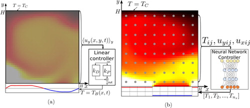
Figure 2. Sketch of the neural network determining the policy adopted by the RL-based controller (policy network, π, cf. Figure 1(b) for the complete setup). The input of the policy network is a state vector, $\mathbf{s}$, which stacks the values of temperature and both velocity components for the current and the previous D−1 = 3 timesteps. Temperature and velocity are read on an evenly spaced grid of size $G_X=8$ by $G_Y=8$. Hence, $\mathbf{s}$ has dimension $n_f\cdot G_X\cdot G_Y\cdot D=3\cdot 8\cdot 8\cdot 4=768$. The policy network π is composed of two fully connected feed forward layers with $n_{\mathrm{neurons}}=64$ neurons and $\sigma (\cdot )=\text{tanh}(\cdot )$ activation. The network output is provided by one fully connected layer with $\sigma (\cdot )=\varphi (\cdot )$ activation (Equation 16(16) $y_k=\varphi (z_k)=\frac{1}{1+\exp (-z_k)},k=1,2,\dots ,n_s$(16) ). This returns the probability vector $\mathbf{y}=[y_1,y_2,\dots ,y_{n_s}]$. The kjth bottom segment has temperature C with probability $y_k$ (Equation 17(17) ${\pi }_k({\tilde{T}}_k=+C|s_i)=\mathrm{Bernoulli}(p=y_k).$(17) ). This probability distribution gets sampled to produce a proposed temperature profile $\tilde{\mathbf{T}}=({\tilde{T}}_1,{\tilde{T}}_2,\dots ,{\tilde{T}}_{n_s})$. The final temperature fluctuations ${\hat{T}}_1,{\hat{T}}_2,\dots ,{\hat{T}}_{n_s}$ are generated with the normalization step in Equation (A7(A7) $\begin{array}{rl}& {\hat{T}}_B(x,t)=\frac{{\tilde{T}}_B^{″}(x,t)}{\underset{x^{\prime }}{max}(1,|{\tilde{T}}_B^{″}(x,t)|/C)}.\end{array}$(A7) ) (cf. Equations (7(7) $T_H=⟨T_B(x,t){⟩}_x,$(7) ) and (9(9) ${\hat{T}}_B(x,t)|\le C\mathrm{\forall }x,t,$(9) )). The temperature profile obtained is applied to the bottom plate during a time interval $\mathrm{\Delta }t$ (control loop), after which the procedure is repeated.

Table 1. Rayleigh–Bénard  system and simulation parameters.

Parameters
$\mathrm{Ra}$	${10}^3\stackrel{}{\to }{10}^7$	Rayleigh Number
$\mathrm{Pr}$	0.71	Prandtl Number
Γ	1	Aspect Ratio
Control
C	0.75	Control amplitude limit, Equation (9(9) ${\hat{T}}_B(x,t)|\le C\mathrm{\forall }x,t,$(9) )
$\mathrm{\Delta }t$	$16\stackrel{}{\to }180$	Control loop (unit: LBM steps)
$t_i$	0 (training)	Start evaluation time, for averages in Equation (5(5) $\mathrm{Nu}=\frac{q}{\kappa \mathrm{\Delta }T/H}.$(5) )
”	$150\mathrm{\Delta }t$ (test)	”
$t_e$	$500\mathrm{\Delta }t$	End evaluation time, for averages in Equation (5(5) $\mathrm{Nu}=\frac{q}{\kappa \mathrm{\Delta }T/H}.$(5) )
Lattice Boltzmann simulation (Appendix 1)
$N_X=N_Y$	$20\stackrel{}{\to }350$	Grid size
$c_s^2$	1/3	Speed of sound
τ	0.56	Relaxation time
$T_C$	1	Top boundary temperature
$T_H$	2	Bottom boundary mean temperature
${\tau }_T$	$(\tau -1/2)/\mathrm{Pr}+1/2$	Temperature relaxation time
ν	$c_s^2(\tau -1/2)$	Kinematic viscosity
κ	$(2{\tau }_T-1)/4$	Thermal diffusivity
$\alpha g$	$\mathrm{Ra}{\displaystyle \frac{\kappa \nu }{(T_H-T_C)N_Y^3}}$	Effective gravity

Table 2. Parameters used for the linear controls in Lattice Boltzmann units (cf. Equation (10(10) ${\hat{T}}_B(x,t)=\mathcal{R}({\tilde{T}}_B(x,t))=-\mathcal{R}((k_P-k_D{\mathrm{\partial }}_t)E(x,t))$(10) ); note: a P controller is obtained by setting $k_D=0$ ). At $\mathrm{Ra}={10}^7$ we were unable to find PD controllers performing better than P controllers, which were anyway ineffective.

		P control	PD control
Ra	$N_x=N_y$	$k_P$	$k_P$	$k_D$
$1\cdot {10}^3$	20	0.0	0.0	0.0
$3\cdot {10}^3$	20	$3.16\cdot {10}^2$	$3.16\cdot {10}^2$	0.0
$1\cdot {10}^4$	20	$4.12\cdot {10}^2$	$5.28\cdot {10}^2$	$8.24\cdot {10}^4$
$3\cdot {10}^4$	25	$8.97\cdot {10}^2$	$5.45\cdot {10}^4$	$1.91\cdot {10}^6$
$1\cdot {10}^5$	30	16.4	94.8	$1.05\cdot {10}^4$
$3\cdot {10}^5$	40	9.38	11.5	$1.87\cdot {10}^3$
$1\cdot {10}^6$	100	6.61	$1.84\cdot {10}^4$	$3.06\cdot {10}^5$
$3\cdot {10}^6$	200	7.38	0.12	31.8
$1\cdot {10}^7$	350	0.33	–	–

Figure 3. Comparison of Nusselt number, averaged over time and ensemble, measured for uncontrolled and controlled Rayleigh–Bénard  systems (note that all the systems are initialised in a natural convective state). We observe that the critical Rayleigh number, $\mathrm{Ra}{}_c$, increases when we control the system, with $\mathrm{Ra}{}_c={10}^4$ in case of state-of-the-art linear control and ${\mathrm{Ra}}_c=3\cdot {10}^4$ in case of the RL-based control. Furthermore, for $\mathrm{Ra}>{\mathrm{Ra}}_c$, the RL control achieves a Nusselt number consistently lower than what measured in case of the uncontrolled system and for state-of-the-art linear controls (P and PD controllers have comparable performance at all the considered Rayleigh numbers, see also [13]). The error bars are estimated as ${\mu }_{\mathrm{Nu}}/\sqrt{N}$, where N = 161 is the number of statistically independent samplings of the Nusselt number.

Figure 4. Time evolution of the Nusselt number at four different Rayleigh regimes, with the control starting at t = 0. The time axis is in units of control loop length, $\mathrm{\Delta }t$ (cf. Table A1). Up to $\mathrm{Ra}=3\cdot {10}^4$ (a,b), the RL control is able to stabilise the system (i.e. $\mathrm{Nu}\approx 1$), which is in contrast with linear methods that result in a unsteady flow. At $\mathrm{Ra}={10}^5$ (c), the RL control is also unable to fully stabilise the system, yet, contrarily to the linear case, it still results in a flow having stationary Nu. For $\mathrm{Ra}={10}^6$ (d) the performance of RL is not as stable as at lower $\mathrm{Ra}$, the control however still manages to reduce the average Nusselt number significantly. (a) $\mathrm{Ra}=1\cdot {10}^4$, (b) $\mathrm{Ra}=3\cdot {10}^4$, (c) $\mathrm{Ra}=1\cdot {10}^5$ and (d) $\mathrm{Ra}=1\cdot {10}^6$.

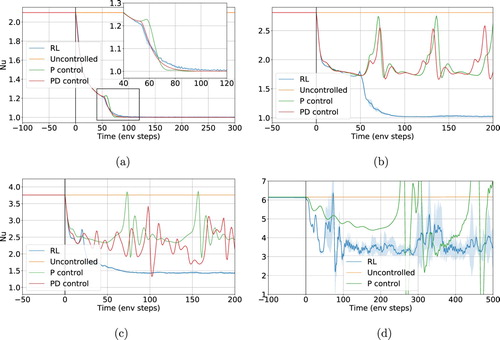
Figure 5. Instantaneous stream lines at different times, at $\mathrm{Ra}={10}^5$, comparison of cases without control (a), with linear control (b) and with RL-based control (c). Note that the time is given in units of $\mathrm{\Delta }t$ (i.e. control loop length, cf. Table A1. Note that the snapshots are taken at different instants). RL controls establish a flow regime like a ‘double cell mode’ which features a steady Nusselt number (see Figure 4c). This is in contrast with linear methods which rather produce a flow with fluctuating Nusselt. The double cell flow field has a significantly lower Nusselt number than the uncontrolled case, as heat transport to the top boundary can only happen via diffusion through the interface between the two cells. This ‘double cell’ control strategy is established by the RL control with any external supervision.

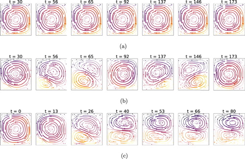
Figure 6. Instantaneous stream lines at $\mathrm{Ra}=3\cdot {10}^6$, comparison of cases without control (a), with linear control (b), and with RL-based control (c). We observe that the RL control still tries to enforce a ‘double cell’ flow, as in the lower Rayleigh case (Figure 5). The structure is, however, far less pronounced and convective effects are much stronger. This is likely due to the increased instability and chaoticity of the system, which increases the learning and controlling difficulty. Yet, we can observe a small alteration in the flow structure (cf. lower cell, larger in size than in uncontrolled conditions) which results in a slightly lower Nusselt number.

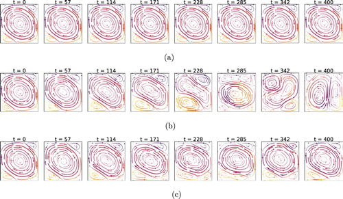
Figure 7. Performance loss due to an artificial delay imposed to an RL controller operating on the Lorenz attractor. The controller, operating on the y variable of the system (reduced model for the RBC horizontal temperature fluctuations) aims at either maximising (LA oscillator) or minimising (LA stabiliser) the number of sign changes of the x (in RBC terms the angular velocity of the flow). The delay, on the horizontal axis, is scaled on the Lyapunov time, ${\lambda }^{-1}$, of the system (with λ the largest Lyapunov exponent). In case of a delay in the control loop comparable in size to the Lyapunov time, the control performance diminishes significantly.

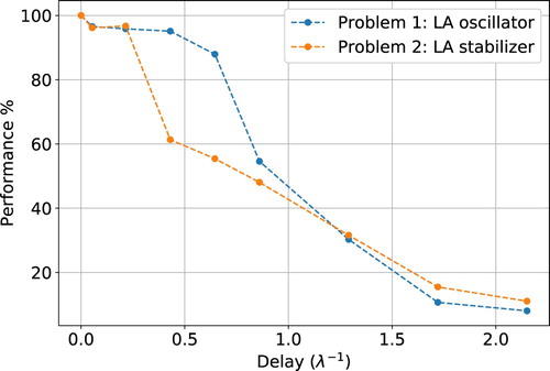
Figure 8. Average Nusselt number for an RL agent observing the Rayleigh–Bénard  environment at different probe density, all of which are lower than the baseline employed in Section 3. The grid sizes (i.e information) used to sample the state of the system at the Ra considered does not seem to play key role in limiting the final control performance of the RL agent.

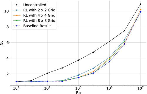
Table A1. Rayleigh–Bénard  environments considered. For each Rayleigh number we report the LBM grid employed (size $N_X\times N_Y$), the uncontrolled Nusselt number measured from LBM simulations and a validation reference from the literature.

Ra	$N_X$ and $N_Y$	Length 1 env step (i.e. control loop length) (units: lbm steps)	Nu	Nu reference [47]
$1\cdot {10}^3$	20	16	1.000	1.000
$3\cdot {10}^3$	20	16	1.141
$1\cdot {10}^4$	20	30	2.090	2.15
$3\cdot {10}^4$	25	60	2.753
$1\cdot {10}^5$	30	60	3.847	3.91
$3\cdot {10}^5$	40	60	4.768
$1\cdot {10}^6$	100	60	6.136	6.3
$3\cdot {10}^6$	200	100	7.500
$1\cdot {10}^7$	350	180	10.900

Figure A1. Performance of RL during training (case of the Rayleigh–Bénard  system). We report the average Nusselt number and its fluctuations computed among a batch of 512 concurrent training environments. (a) ‘low’ Ra ($0\lesssim \mathrm{Ra}\lesssim 3\cdot {10}^4$) in which the control achieves $\mathrm{Nu}\approx 1$ in a stable way, (b)‘mid’ Ra ($3\cdot {10}^4\lesssim \mathrm{Ra}\lesssim 1\cdot {10}^6$) which still gives stable learning behaviour but converges to $\mathrm{Nu}>1$ and, lastly, (c) ‘high’ Ra ($1\cdot {10}^6\lesssim \mathrm{Ra}$) in which the higher chaoticity of the system makes a full stabilization impossible. (a) $\mathrm{Ra}=3\cdot {10}^4$ (‘low’). (b) $\mathrm{Ra}=3\cdot {10}^5$ (‘mid’) and (c) $\mathrm{Ra}=3\cdot {10}^6$ (‘high’).

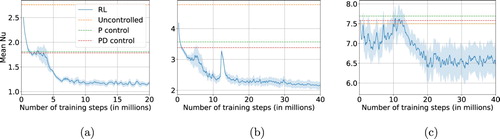
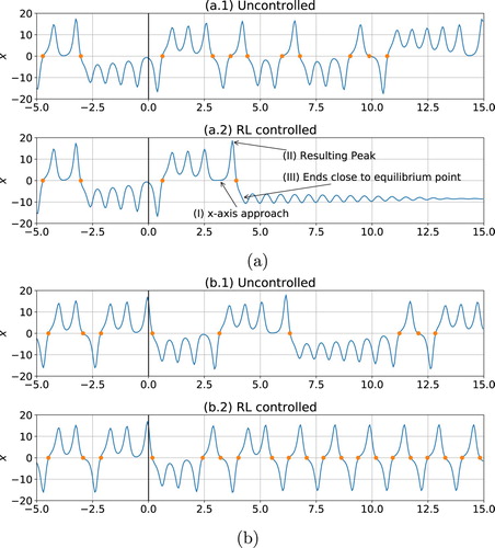
Figure A2. System trajectories with RL control, respectively aiming at minimising (a) and maximising (b) the number of x sign changes. In (a.1) and (b.1), we report two reference uncontrolled cases which differ only by the initialization state, $x(-5),y(-5),z(-5)$. Panel (a) shows that the RL agent is able to fully stabilise the system on an unstable equilibrium by using a complex strategy in three steps (I: controlling the system such that it approaches x, y, z = 0 which results in a peak (II) which after going through x = 0 ends close enough to an unstable equilibrium (III) such that the control is able to fully stabilise the system). Furthermore, Figure 2(a) shows that the RL agent is able to find and stabilise a unstable periodic orbits with a desired property of a high frequency of sign changes of x.

Remillieux MC, Zhao H, Bau HH. Suppression of Rayleigh–Bénard convection with proportional-derivative controller. Phys Fluids. 2007;19(1):017102. doi: 10.1063/1.2424490

 Web of Science ®Google Scholar

Ouertatani N, Cheikh NB, Beya BB, et al. Numerical simulation of two-dimensional Rayleigh–Bénard convection in an enclosure. Comp Rend Mécaniq. 2008;336(5):464–470. doi: 10.1016/j.crme.2008.02.004

 Web of Science ®Google Scholar