Build up of yield stress fluids via chaotic emulsification

Figures & data

Table 1. Main parameters and relevant observables for all simulations, labelled by a ${\mathrm{RUN}}_{\mathrm{id}}$, presented in this paper: system size, L, (the grid spacing in all three directions is set to unity); energy injection rate, $E_{\mathrm{in}}=\overline{\mathbf{f}\cdot \mathbf{v}}$; root mean square velocity, $V_{\mathrm{rms}}=\sqrt{\overline{|\mathbf{v}{|}^2}}$; $T_L=L/V_{\mathrm{rms}}$ is the large-scale correlation time; ${\tau }_{\varphi }$ is the inverse injection rate; average number of droplets, $\overline{N_D}$; volume mean radius, $R_{30}=\sqrt[3]{\frac{3}{4\pi }⟨V_D⟩}$ ($V_D$ is the droplet volume); arithmetic mean radius, $R_{10}=⟨R⟩$; standard deviation of droplet radii, $R_{\sigma }$; capillary number, $Ca=\frac{\rho \nu V_{\mathrm{rms}}}{\sigma }$; Weber number, $We=\frac{\rho R_{10}{V}_{\mathrm{rms}}^2}{\sigma }$; Reynolds number as $Re=\frac{L{V}_{\mathrm{rms}}}{\nu }$.

${\mathrm{RUN}}_{\mathrm{id}}$	L	$E_{\mathrm{in}}$	$V_{\mathrm{rms}}$	$T_L$	${\tau }_{\varphi }/T_L$	$\overline{N_D}$	$R_{30}$	$R_{10}$	$R_{\sigma }$	Ca	We	Re
A	256	$7.196\cdot {10}^{-8}$	0.0115	22261	35.9	112.7	30.1	26.7	9.50	0.109	0.227	123.47
B	512	$6.294\cdot {10}^{-8}$	0.0178	28764	27.8	877.2	30.4	27.9	8.42	0.169	0.548	381.79
C	1024	$6.597\cdot {10}^{-8}$	0.0312	32821	24.4	5707.1	32.6	28.4	11.03	0.296	1.809	1339.27

Note: $\rho =1.36$ is the total fluid density, $\nu =c_s^2({\tau }_{\mathrm{LB}}-0.5)=1/6$ is the kinematic viscosity, equal for both pure fluids ($c_s=1/\sqrt{3}$ is the speed of sound and ${\tau }_{\mathrm{LB}}=1$ is the lattice Boltzmann relaxation time), and $\sigma =0.0238$ is the surface tension. The averages, $\overline{(\cdots )}$, are taken over time, in the interval $T_3$ (where the final concentration of the emulsion is achieved but the emulsion is still stirred), whereas the averages $⟨(\cdots )⟩$ are meant to taken over time and number of droplets.

Figure 1. Graphical illustration of the emulsification process via large-scale stirring and slow injection of the dispersed phase. Snapshots of the interface (red/blue side corresponding to the continuous/dispersed phase) during stirring at various instants of time (given in units of the large-scale characteristic time $T_L=L/V_{\mathrm{rms}}$, where $V_{\mathrm{rms}}$ is computed once the injection process is terminated, i.e. at the maximum volume fraction; see also Figure 3 and caption therein). Both time and the volume fraction of the dispersed phase ϕ grow from (a)–(j). Panel (a): the slightly deformed initially flat interface is still clearly visible, no droplets have formed yet. Panels (b)–(d): the process of fragmentation of the initial interface, leading to the production of a large number of small droplets, can be appreciated (see e.g. panel (d)). Panels (e)–(j): ϕ further increases, droplets become smaller and the system becomes more and more densely packed. The simulation parameters are reported in Table 1 (run C). (a) $\varphi =30\mathrm{\%}$ $t=0.6T_L$ (b) $\varphi =31\mathrm{\%}$ $t=1.2T_L$ (c) $\varphi =32\mathrm{\%}$ $t=1.8T_L$ (d) $\varphi =33\mathrm{\%}$ $t=2.4T_L$ (e) $\varphi =35\mathrm{\%}$ $t=3T_L$ (f) $\varphi =42\mathrm{\%}$ $t=6T_L$ (g) $\varphi =50\mathrm{\%}$ $t=9T_L$ (h) $\varphi =60\mathrm{\%}$ $t=12T_L$ (i) $\varphi =70\mathrm{\%}$ $t=15T_L$ (j) $\varphi =77\mathrm{\%}$ $t=18T_L$.

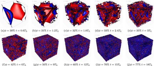
Figure 2. Snapshot of the final interface field configuration from simulations with volume fraction $\varphi =77\mathrm{\%}$ (panel (a)) and $\varphi =28\mathrm{\%}$ (panel (b)). As it can be observed, at the largest volume fraction the droplets are highly deformed, while at lower volume fraction they preserve their equilibrium spherical shape and their average size is smaller. (a) ${512}^3$ – $\varphi =77\mathrm{\%}$ (b) ${512}^3$ – $\varphi =28\mathrm{\%}$.

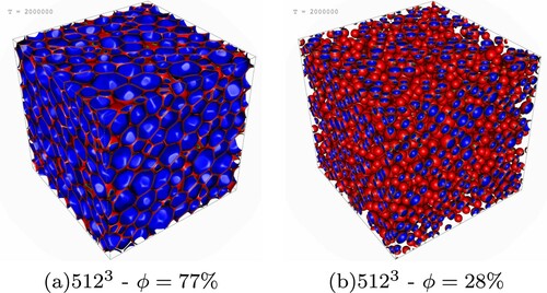
Figure 3. MAIN PANEL. Number density of droplets, $N_D/L^3$, as a function of time for different resolutions: L = 256 (red squares, $◻$), L = 512 (green circles, °) and L = 1024 (blue triangles, $\mathrm{△}$). The volume fraction of the dispersed phase, $\varphi (t)$, as a function of time is also reported on the $y2$-axis (magenta crosses, ×), together with an exponential fit in the injection phase $T_0+T_1+T_3$ (dashed line). The time is given in units of ${\tau }_{\varphi }$, the inverse injection rate (i.e. such that the total mass of dispersed phase fulfils $\dot{M}(t)={\tau }_{\varphi }^{-1}M(t)$). Further details on the parameter used in the simulations are provided in Table 1. INSET: Zoom on the first time window ($T_0$) in logarithmic scale on the y-axis to highlight the initial exponential increase of the number of droplets (the dashed line represents the exponential fit, drawn as a guide to the eye).

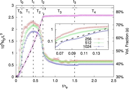
Figure 4. PDFs $P_{\tau }(R)$ (from the simulation C, see Table 1) of the effective droplet radii (i.e. for each droplet, the radius of the equivalent sphere is measured) given in units of the mean volume radius $R_{30}$, computed in four different time windows, τ. During the initial phase, $\tau \subset T_0$, the process of stirring-induced interface fragmentation dominates and the PDF displays a peak at $R\approx 0.15R_{30}$, followed by the typical slope $\sim R^{-10/3}$ (panel (a)). As the concentration of the dispersed phase increases, for $\tau \subset T_1$ a steeper decay, $\sim R^{-6}$, develops for large sizes, the change of slop occurring at $R\approx R_{30}$; in parallel, the peak is shifted towards higher R (panel (b)). Eventually, when the injection procedure is completed and the volume fraction of dispersed phase is $\approx 77\mathrm{\%}$, the peak merges with the bend at $R\approx R_{30}$ and a secondary peak emerges again at $R\approx 0.15R_{30}$, giving $P_{\tau }(R)$ (for $\tau \subset T_3$) a bimodal shape, evidence of the increasing presence of small droplets (panel (c)). This secondary maximum tends to vanish when the forcing is switched off (panel (d)).

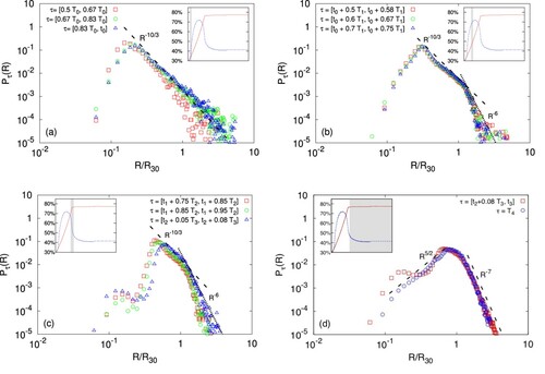
Figure 5. Time evolution of the number of droplets from a simulation of a system which eventually undergoes a catastrophic phase inversion: the red thick line indicates the droplets number for the ‘fluid 1’, $N_D^{(1)}$, namely the initially dispersed phase which gets progressively concentrated, whereas the blue thin line indicates $N_D^{(2)}$, the droplets number for ‘fluid 2’, the initially continuous phase; the black dashed line shows the growth of the volume fraction of ‘fluid 1’, ϕ. The two snapshots highlights the density field from configurations at two instants of time (indicated by the black arrows), respectively before and after the catastrophic phase inversion.

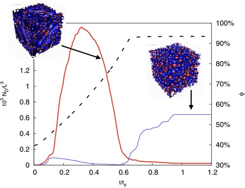
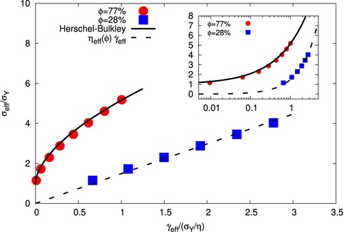
Figure 6. (Main panel) Flow curves for the emulsions with $\varphi =77\mathrm{\%}$ (red bullets) and $\varphi =28\mathrm{\%}$ (blue squares), showing effective shear stress, ${\sigma }_{\mathrm{eff}}$ (normalized with the yield stress ${\sigma }_Y$), vs effective shear rate, ${\dot{\gamma }}_{\mathrm{eff}}$ (normalized with the yield stress divided by the dynamics viscosity ${\sigma }_Y/\eta$), as defined in Equations (3(3) ${\sigma }_{\mathrm{eff}}=⟨{\sigma }^2{⟩}^{1/2}=\left(\frac{L}{2\pi }\right)\frac{F}{\sqrt{2}}$(3) )–(4(4) ${\dot{\gamma }}_{\mathrm{eff}}\equiv \frac{⟨\sigma (y)\dot{\gamma }(y)⟩}{⟨{\sigma }^2(y){⟩}^{1/2}},$(4) ). The solid line indicates a Herschel–Bulkley fit, $\sigma ={\sigma }_Y+K{\dot{\gamma }}^{\beta }$, with ${\sigma }_Y=2.5\times {10}^{-5}$ lbu, K = 0.02 lbu, $\beta =0.58$, whereas the dashed line represents the Newtonian relation $\sigma ={\eta }_{\mathrm{eff}}\dot{\gamma }$, with an effective viscosity compliant with the Taylor's prediction for equiviscous, low concentrated, emulsions, namely ${\eta }_{\mathrm{eff}}(\varphi )=\eta (1+(7/4)\varphi )$. (Inset) Same as in the main panel but in log-log scale.