Effect of high skewness and kurtosis on turbulent channel flow over irregular rough walls

Figures & data

Figure 1. Map of skewness-kurtosis combinations reported for irregular engineering rough surfaces (black circles) adapted from Jelly & Busse [8]. The black line shows the boundary of Pearson's inequality (1(1) $Ss{k}^2-Sku+1\le 0$(1) ). The red squares show the skewness-kurtosis combinations investigated in the current study. The blue dotted line gives the boundary of possible skewness-kurtosis combinations for unimodal distributions (3(3) $Ss{k}^2-Sku+\frac{189}{125}\le 0.$(3) ).

Figure 2. Visualisations of the generated irregular rough surfaces. First row: Gaussian reference surface; second row: negatively skewed surfaces from left to right in order of increasing $⏐Ssk⏐$; third row: positively skewed surfaces from left to right in order of increasing Ssk.

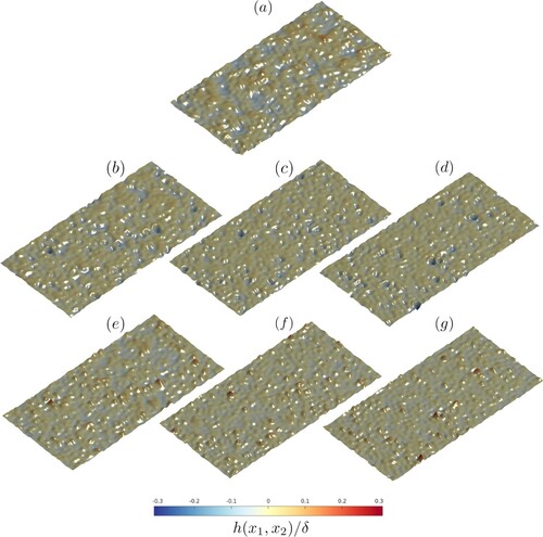
Figure 3. (a) Probability density functions and (b) cumulative distribution functions of $h(x,y)$ of the surfaces shown in Figure 2. Line styles are given in Table 2. The inset plots show the same data with a logarithmic y-axis.

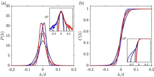
Table 1. Key topographical parameters of the surfaces investigated in the current DNS.

Name	$Sa/\delta$	$Sq/\delta$	$S{z}_{5\times 5}/\delta$	Ssk	Sku	$E{S}_x$	$E{S}_y$	$S_{max}/\delta$	$S_{min}/\delta$
Gaussian	0.0263	0.0330	0.167	0.0	3.0	0.209	0.220	$+0.1429$	$-0.0996$
skew_p1p0	0.0205	0.0269	0.167	$+1.0$	5.8	0.204	0.207	$+0.2239$	$-0.0735$
skew_m1p0	0.0205	0.0269	0.167	$-1.0$	5.8	0.204	0.207	$+0.0735$	$-0.2239$
skew_p1p5	0.0173	0.0234	0.167	$+1.5$	8.0	0.204	0.203	$+0.2126$	$-0.0605$
skew_m1p5	0.0173	0.0234	0.167	$-1.5$	8.0	0.204	0.204	$+0.0605$	$-0.2126$
skew_p2p3	0.0168	0.0237	0.167	$+2.3$	17.0	0.198	0.195	$+0.3044$	$-0.0749$
skew_m2p3	0.0168	0.0237	0.167	$-2.3$	17.0	0.198	0.195	$+0.0749$	$-0.3044$

Notes: Sa – mean roughness height; Sq – rms roughness height; $S{z}_{5\times 5}$ mean peak-to-valley height; Ssk – surface skewness; Sku – surface kurtosis; $E{S}_x$ – streamwise effective slope; $E{S}_y$ – spanwise effective slope; $S_{max}$ - maximum height; $S_{min}$ – minimum height.

Table 2. Simulation parameters for the current rough-wall channel flow DNS.

case	$L_1$	$L_2$	$L_3$	$n_1\times n_2\times n_3$	$\mathrm{\Delta }{x}_1^{+}$	$\mathrm{\Delta }{x}_2^{+}$	$\mathrm{\Delta }{x}_{3,min}^{+}$	$\mathrm{\Delta }{x}_{3,max}^{+}$	line style
Gaussian	8	4	2	$640\times 320\times 576$	4.94	4.94	0.667	4.04	$\text{-}$
skew_p1p0	8	4	2	$640\times 320\times 576$	4.94	4.94	0.667	4.92	$red\text{–}$
skew_m1p0	8	4	2	$640\times 320\times 624$	4.94	4.94	0.667	4.80	$blue\text{‐}$
skew_p1p5	8	4	2	$640\times 320\times 576$	4.94	4.94	0.667	4.66	$red\text{‐}$
skew_m1p5	8	4	2	$640\times 320\times 624$	4.94	4.94	0.667	4.59	$blue\text{‐}$
skew_p2p3	8	4	2	$640\times 320\times 672$	4.94	4.94	0.667	4.40	$red\text{-}$
skew_m2p3	8	4	2	$640\times 320\times 720$	4.94	4.94	0.667	4.96	$blue\text{-}$
smooth	8	4	2	$640\times 320\times 360$	4.94	4.94	0.50	3.98	$\circ \circ \circ \circ$

Notes: $L_1$: streamwise domain size; $L_2$: spanwise domain size; $L_3$: mean channel height; $n_1\times n_2\times n_3$: number of grid points; $\mathrm{\Delta }{x}_1^{+}$: grid-spacing in streamwise direction; $\mathrm{\Delta }{x}_2^{+}$ grid-spacing in spanwise direction; $\mathrm{\Delta }{x}_{3,min}^{+}$: minimum wall-normal grid-spacing; $\mathrm{\Delta }{x}_{3,max}^{+}$: maximum wall-normal grid-spacing.

Figure 4. (a) Mean streamwise velocity profile; the inset shows the local downwards shift, i.e. the difference between the smooth-wall and the rough-wall velocity profile vs the wall-normal coordinate; (b) Velocity defect profile; the inset shows the difference between the smooth-wall and rough-wall velocity defect profile. Line styles are given in Table 2.

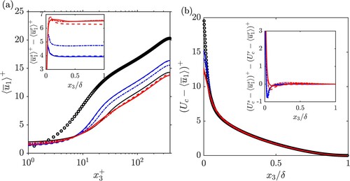
Figure 5. (a) Roughness function vs surface skewness. The black dashed line shows the fit given in Equation (21(21) $\mathrm{\Delta }{U}^{+}=a\mathrm{t}\mathrm{a}\mathrm{n}\mathrm{h}(Ssk+b)+c$(21) ). (b) Estimated equivalent sand-grain roughness normalised by rms roughness height vs skewness. The corresponding behaviour predicted by the empirical relationship (22(22) $k_s=\alpha Sq(\gamma +Ssk{)}^{\text{β}},\mathrm{w}\mathrm{h}\mathrm{e}\mathrm{r}\mathrm{e}\{\begin{array}{lr}\alpha =2.48,\text{β}=2.24,\gamma =1& \mathrm{f}\mathrm{o}\mathrm{r}Ssk>0,\\ \alpha =2.11,\text{β}=0,\gamma =1& \mathrm{f}\mathrm{o}\mathrm{r}Ssk=0,\\ \alpha =2.73,\text{β}=-0.45,\gamma =2& \mathrm{f}\mathrm{o}\mathrm{r}Ssk<0.\end{array}$(22) ) is also shown - blue line: negative skewness branch; red line: positive skewness branch; black cross: neutral skewness condition.

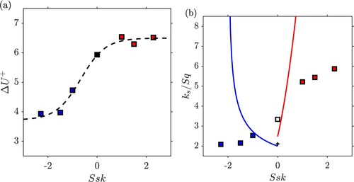
Table 3. Mean flow quantities measured for the present surfaces.

case	$U_c$	$\overline{U}$	${\text{Re}}_c$	$\text{Re}$	$\mathrm{\Delta }{U}^{+}$	$F_p/F_{tot}$
Gaussian	14.30	11.73	5,647	9,267	5.93	0.53
skew_p1p0	13.72	11.51	5,421	8,810	6.54	0.53
skew_m1p0	15.55	12.86	6,144	10,160	4.73	0.47
skew_p1p5	14.01	11.34	5,534	8,972	6.29	0.51
skew_m1p5	16.32	13.60	6,445	10,744	3.97	0.44
skew_p2p3	13.76	11.17	5,436	8,824	6.52	0.54
skew_m2p3	16.37	13.63	6,465	10,773	3.93	0.43
smooth	20.92	17.57	8,015	13,882	–	0.0

Notes: $U_c$: centreline velocity; $\overline{U}$: bulk flow velocity; ${\text{Re}}_c=\delta U_c/\nu$: Reynolds number based on centreline velocity; $\text{Re}=2\delta \overline{U}/\nu$: Reynolds number based on bulk flow velocity; $\mathrm{\Delta }{U}^{+}$: roughness function; $F_p/F_{tot}$ fractional pressure drag contribution.

Figure 6. (a) Streamwise Reynolds stresses; (b) streamwise dispersive stresses; line styles are given in Table 2. The abscissae have been clipped to the range $[-0.2,1.0]$. The inset plots show the maxima as a function of the surface skewness Ssk.

Figure 7. Visualisations of time-averaged streamwise velocity in plane $x_3/\delta =0.05$. First row: Gaussian reference surface; second row: negatively skewed surfaces from left to right in order of increasing $⏐Ssk⏐$; third row: positively skewed surfaces from left to right in order of increasing Ssk.

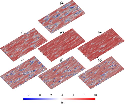
Figure 8. (a) Spanwise Reynolds stresses; (b) spanwise dispersive stresses; line styles are given in Table 2. The abscissae have been clipped to the range $[-0.2,1.0]$. The inset plots show the maxima as a function of the surface skewness Ssk.

Figure 9. (a) Wall-normal Reynolds stresses; (b) wall-normal dispersive stresses; line styles are given in Table 2. The abscissae have been clipped to the range $[-0.2,1.0]$. The inset plots show the maxima as a function of the surface skewness Ssk. For the dispersive stress case, the maximum values are based on the outer maxima ($max(〈{\tilde{u}}_3{\tilde{u}}_3〉(x_3>0\left)\right)$).

Figure 10. (a) Reynolds shear stress; (b) dispersive shear stress; line styles are given in Table 2. The abscissae have been clipped to the range $[-0.2,1.0]$. The inset plots show the maxima as a function of the surface skewness Ssk.

Figure 11. Fractional contribution of pressure drag vs (a) surface skewness and (b) Hama roughness function. The grey triangles show data for a pit-peak decomposed surface ($Ssk=\pm 1.62$, $E{S}_x=0.17$) [12] for comparison.

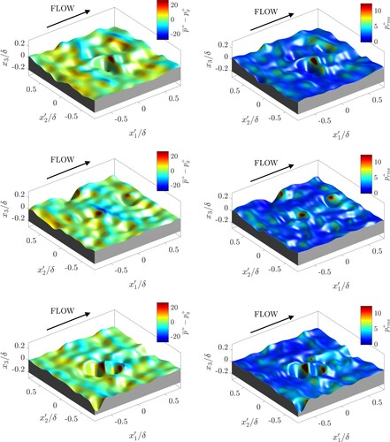
Figure 12. Surface pressure distributions for $Ssk\ge 0$ centred about the highest peak. Left column: time-averaged pressure on surface; right column: time-averaged pressure fluctuations at surface. From top to bottom: Ssk = +2.3, Ssk = +1.5, Ssk = +1.0, and Ssk = 0.0.

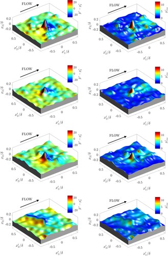
Figure 13. Surface pressure distributions for Ssk<0 centred about the highest peak. Left column: time-averaged pressure on surface; right column: time-averaged pressure fluctuations at surface. From top to bottom: Ssk = −1.0, Ssk = −1.5, and Ssk = −2.3.

Jelly TO, Busse A. Reynolds number dependence of Reynolds and dispersive stresses in turbulent channel flow past irregular near-Gaussian roughness. Int J Heat Fluid Flow. 2019;80:108485.

 Web of Science ®Google Scholar

Jelly TO, Busse A. Reynolds and dispersive stress contributions above highly skewed roughness. J Fluid Mech. 2018;852:710–724.

 Web of Science ®Google Scholar