
Figures & data
Figure 1. Left: Virginia Tech 2D smooth wall flow (2D VT) (from [Citation11]; reprinted by permission of the American Institute of Aeronautics and Astronautics, Inc.). Right: DLR/UniBw 2D smooth wall flow (reprinted with permission from [Citation16]).
![Figure 1. Left: Virginia Tech 2D smooth wall flow (2D VT) (from [Citation11]; reprinted by permission of the American Institute of Aeronautics and Astronautics, Inc.). Right: DLR/UniBw 2D smooth wall flow (reprinted with permission from [Citation16]).](/cms/asset/352fb847-752d-4051-b00a-91148ed969cc/tjot_a_2360195_f0001_oc.jpg)
Figure 2. Left: 3D BeVERLI Hill flow (from [Citation17]; reprinted by permission of the American Institute of Aeronautics and Astronautics, Inc.). Right: Body-of-Revolution in turbulent flow.
![Figure 2. Left: 3D BeVERLI Hill flow (from [Citation17]; reprinted by permission of the American Institute of Aeronautics and Astronautics, Inc.). Right: Body-of-Revolution in turbulent flow.](/cms/asset/adadb8a7-96c8-403e-b51f-79144c65a1f6/tjot_a_2360195_f0002_oc.jpg)
Figure 3. Left: Grid metrics using arithmetic average and root-mean-square cell areas for the grid levels for the 2D VT flow. Right: Grid levels 1, 3, 5 showing hierarchical refinement (zoom of the mesh for the 2D VT flow)(Figures from [Citation11]; reprinted by permission of the American Institute of Aeronautics and Astronautics, Inc.).
![Figure 3. Left: Grid metrics using arithmetic average and root-mean-square cell areas for the grid levels for the 2D VT flow. Right: Grid levels 1, 3, 5 showing hierarchical refinement (zoom of the mesh for the 2D VT flow)(Figures from [Citation11]; reprinted by permission of the American Institute of Aeronautics and Astronautics, Inc.).](/cms/asset/71488c91-131d-4719-ad5f-44945b973c74/tjot_a_2360195_f0003_oc.jpg)
Figure 4. Convergence study for 2D VT flow. Left: Mesh convergence for using the SST model using the CFD solver Kestrel. Middle and right: Code to code comparison for
and mean velocity profiles
vs.
on grid level 3(Figures from [Citation11]; reprinted by permission of the American Institute of Aeronautics and Astronautics, Inc.).
![Figure 4. Convergence study for 2D VT flow. Left: Mesh convergence for Cf using the SST model using the CFD solver Kestrel. Middle and right: Code to code comparison for Cf and mean velocity profiles u+ vs. y+ on grid level 3(Figures from [Citation11]; reprinted by permission of the American Institute of Aeronautics and Astronautics, Inc.).](/cms/asset/723de69a-1809-49ed-9a0b-84d0455cf50c/tjot_a_2360195_f0004_oc.jpg)
Figure 5. Illustration of the impact of an adjusted computational set-up compared to the original set-up for the 2D DLR/UniBw flow for the displacement thickness along the contour (left) and for the mean velocity profile in the region of strong adverse pressure gradient at
(right).
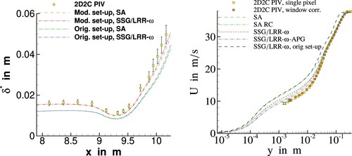
Figure 6. and
along the centerline in the streamwise
-direction (left) and the centerspan in the spanwise
-direction (right) from the
yaw case BeVERLI Hill at
on grid levels GL1 to GL4 (from [Citation13]; reprinted by permission of the American Society of Mechanical Engineers ASME). Note that
and
in Figure (left). The dotted line shows the hill geometry.
![Figure 6. Cp and Cf along the centerline in the streamwise x1-direction (left) and the centerspan in the spanwise x3-direction (right) from the 45∘ yaw case BeVERLI Hill at ReH≈650,000 on grid levels GL1 to GL4 (from [Citation13]; reprinted by permission of the American Society of Mechanical Engineers ASME). Note that x1≡x and x3≡z in Figure 2 (left). The dotted line shows the hill geometry.](/cms/asset/7765ce4f-1d4d-4259-8b4a-89c09fccdc3a/tjot_a_2360195_f0006_oc.jpg)
Figure 7. Uncertainty due to the discretisation error (DE) in along the centerline in
-direction (top) and the centerspan in
-direction (bottom) of the
yaw case BeVERLI Hill at
for SA-model (left) and SST-model (right) (from [Citation13]; reprinted by permission of the American Society of Mechanical Engineers ASME). Note that
and
in Figure (left). The dotted line shows the hill geometry.
![Figure 7. Uncertainty due to the discretisation error (DE) in Cf along the centerline in x1-direction (top) and the centerspan in x3-direction (bottom) of the 45∘ yaw case BeVERLI Hill at ReH≈650,000 for SA-model (left) and SST-model (right) (from [Citation13]; reprinted by permission of the American Society of Mechanical Engineers ASME). Note that x1≡x and x3≡z in Figure 2 (left). The dotted line shows the hill geometry.](/cms/asset/3857afd7-1844-4cec-ac93-d94efa74bf61/tjot_a_2360195_f0007_oc.jpg)
Figure 8. Left: Uncertainty bars of the discretisation error for for the SST model for two different families of meshes (baseline meshes by VT and meshes with refinement around the airfoil by MARIN/IST (MI)). Right: Estimate of the error of the turbulence model
for
with reference model SST 2003 for model-scale
and for full-scale
(Figures reprinted from [Citation34]).
![Figure 8. Left: Uncertainty bars of the discretisation error for Cf for the SST model for two different families of meshes (baseline meshes by VT and meshes with refinement around the airfoil by MARIN/IST (MI)). Right: Estimate of the error of the turbulence model δtm for Cf with reference model SST 2003 for model-scale Re=2×10⁶ and for full-scale Re=109(Figures reprinted from [Citation34]).](/cms/asset/182f1532-cbbb-4d47-9dc5-2285c39ec833/tjot_a_2360195_f0008_oc.jpg)
Figure 9. Mean velocity profiles in viscous units for the 2D VT flow at model-scale and at full scale
at
for the airfoil incidence angles
(left),
(middle), and
(right)(Figures reprinted from [Citation34]).
![Figure 9. Mean velocity profiles in viscous units for the 2D VT flow at model-scale Re=2×10⁶ and at full scale Re=109 at x=3.5m for the airfoil incidence angles α=−10∘ (left), α=0∘ (middle), and α=12∘ (right)(Figures reprinted from [Citation34]).](/cms/asset/117b3ec8-1f7e-493f-9066-9883a634cf2e/tjot_a_2360195_f0009_oc.jpg)