Unconventional fractional quantum Hall effect in monolayer and bilayer graphene

Figures & data

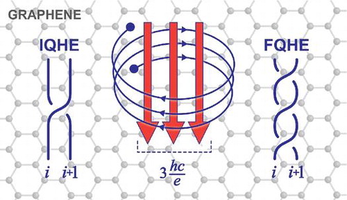
Figure 1. Schematic demonstration that commensurability (left) of cyclotron orbit with interparticle separation satisfies topology requirements for braid interchanges in uniformly and equidistantly (due to interaction) distributed 2D particles; for smaller cyclotron radii particles cannot be matched (center), for larger ones the interparticle distance cannot be conserved (right).

Figure 2. Schematic illustration of cyclotron orbit enhancement in 2D due to multi-loop trajectory structure (third dimension added for visual clarity).

Figure 3. The braid generator ${\mathit{\sigma }}_i$ corresponds to the single exchange of particles (left), the cyclotron orbit (relative) corresponds to the double exchange (right), for (a) $\mathit{\nu }=1$ when single-looped cyclotron trajectory reaches neighboring particles, $R_c=R_o$; and (b) braid generator ${\mathit{\sigma }}_i^3$ for $\mathit{\nu }=\frac{1}{3}$ with additional loop needed for $R_c=R_o$ ($R_c$ is cyclotron radius, $2R_o$ is particle separation, i.e. $\mathit{\pi }{R}_c^2=\frac{hc}{eB}$, $\mathit{\pi }{R}_o^2=\frac{S}{N}$).

Figure 4. Evolution of fractional filling hierarchy in three first LLs of the monolayer graphene; for each LL the first particle subband is illustrated, the next subbands in each LL repeat the hierarchy from the first one. Different types of ordering are indicated with spikes of various height. Series for ordinary FQHE(multiloop), FQHE(single-loop), Hall metal and paired state are displayed according to the hierarchy described in Table 1 with $q=3-9$, $1=1-10$; only a few selected ratios from these series are explicitly written out.

Table 1. LL filling factors for FQHE determined by commensurability condition (paired indicates condensate of electron pairs), for the first particle subband in each of the three first LLs ($n=0,1,2$) for the monolayer graphene.; subb. stands for subband.

LL subb.	FQHE(single-loop), paired, IQHE	FQHE(multiloop) ($q-odd$, $l=\frac{i}{2n+1}$, $i=1,2,3,\cdots$)	Hall metal
$n=0,2\uparrow$	1	$\frac{1}{q},1-\frac{1}{q},\frac{l}{l(q-1)\pm 1},1-\frac{l}{l(q-1)\pm 1}$	$\frac{1}{q-1},1-\frac{1}{q-1}$
$n=1,1\uparrow$	$\frac{7}{3}$, $\frac{8}{3}$, ($\frac{5}{2}paired$), 2, 3	$2+\frac{1}{3q}$, $3-\frac{1}{3q}$, $2+\frac{l}{3l(q-1)\pm 1}$, $3-\frac{l}{3l(q-1)\pm 1}$	$2+\frac{1}{3(q-1)}$, $3-\frac{1}{3(q-1)}$
$n=2,1\uparrow$	$\frac{31}{5}$, $\frac{32}{5}$, $\frac{33}{5}$, $\frac{34}{5}$, ($\frac{13}{2}paired$), 6, 7	$6+\frac{1}{5q}$, $7-\frac{1}{5q}$, $6+\frac{l}{5l(q-1)\pm 1}$, $7-\frac{l}{5l(q-1)\pm 1}$	$6+\frac{1}{5(q-1)}$, $7-\frac{1}{5(q-1)}$

Table 2. LL filling factors for FQHE determined by commensurability condition (paired indicates condensate of electron pairs), for the first particle subband in each of the two first LLs ($n=0,1$ for the extra degenerated LLL and $n=2$ for the first LL beyond the LLL) for the bilayer graphene.

LL subb.	FQHE(single-loop), paired, IQHE	FQHE(multiloop) ($q-odd$, $l=\frac{i}{2n+1}$, $i=1,2,3,\cdots$)	Hall metal
$n=0,2\uparrow$ (LLL)	1	$\frac{1}{(q-1)}$, $1-\frac{1}{(q-1)}$, $\frac{l}{l(q-2)\pm 1}$, $1-\frac{l}{l(q-2)\pm 1}$	$\frac{1}{q-2}$,$1-\frac{1}{q-2}$
$n=1,2\uparrow$ (LLL)	$\frac{7}{3}$, $\frac{8}{3}$, ($\frac{5}{2}paired$), 2, 3	$2+\frac{1}{3(q-1)}$, $3-\frac{1}{3(q-1)}$, $2+\frac{l}{3l(q-2)\pm 1}$, $3-\frac{l}{3l(q-2)\pm 1}$	$2+\frac{1}{3(q-2)}$, $3-\frac{1}{3(q-2)}$
$n=2,1\uparrow$ (first LL)	$\frac{21}{5}$, $\frac{22}{5}$, $\frac{23}{5}$, $\frac{24}{5}$, ($\frac{9}{2}paired$), 4, 5	$4+\frac{1}{5(q-1)}$, $4+\frac{l}{5l(q-2)\pm 1}$, $5-\frac{1}{5(q-1)}$, $5-\frac{l}{5l(q-2)\pm 1}$	$4+\frac{1}{5(q-2)}$, $5-\frac{1}{5(q-2)}$

Table 3. Comparison of filling hierarchy in the LLL level in the bilayer graphene for two mutually inverted successions of two lowest subbands: $n=0,2\uparrow$, $n=1,2,\uparrow$ (upper) and $n=1,2\uparrow$, $n=0,2\uparrow$ (lower).

LL subb.	FQHE(single-loop), paired, IQHE	FQHE(multiloop) ($q-odd$, $l=\frac{i}{2n+1}$, $i=1,2,3,\cdots$)	Hall metal
$n=0,2\uparrow$	1	$\frac{1}{(q-1)}$, $1-\frac{1}{(q-1)}$, $\frac{l}{l(q-2)\pm 1}$, $1-\frac{l}{l(q-2)\pm 1}$	$\frac{1}{q-2}$, $1-\frac{1}{q-2}$
$n=1,2\uparrow$	$\frac{4}{3}$, $\frac{5}{3}$, ($\frac{3}{2}paired$), 1, 2	$1+\frac{1}{3(q-1)}$, $2-\frac{1}{3(q-1)}$, $1+\frac{l}{3l(q-2)\pm 1}$, $2-\frac{l}{3l(q-2)\pm 1}$	$1+\frac{1}{3(q-2)}$, $2-\frac{1}{3(q-2)}$
$n=1,2\uparrow$	$\frac{1}{3}$, $\frac{2}{3}$, ($\frac{1}{2}paired$), 1	$\frac{1}{3(q-1)}$, $1-\frac{1}{3(q-1)}$, $\frac{l}{3l(q-2)\pm 1}$, $1-\frac{l}{3l(q-2)\pm 1}$	$\frac{1}{3(q-2)}$, $1-\frac{1}{3(q-2)}$
$n=0,2\uparrow$	1,2	$1+\frac{1}{q-1}$, $1+\frac{l}{l(q-1)\pm 1}$, $2-\frac{1}{q-1}$, $2-\frac{l}{l(q-2)\pm 1}$	$1+\frac{1}{q-2}$, $2-\frac{1}{q-2}$

Figure 5. Evolution of fractional filling hierarchy in the two first LLs of the bilayer graphene; for the LLL two subbands with $n=0$ and $n=1$ are illustrated. Different types of ordering are indicated with spikes of various heights. Series for ordinary FQHE(multiloop), FQHE(single-loop), Hall metal and paired state are displayed according to the hierarchy described in Table 2 with $q=3-9$, $i=1-10$; only a few selected ratios from these series are explicitly written out.

Figure 6. (a) FQHE observation in suspended graphene for the filling 0.3 (1 / 3) in a field of 12–14 T with the concentration of ${10}^{11}$ cm${}^{-2}$ and the mobility of 250,000 cm${}^2$V${}^{-1}$s${}^{-1}$; (b) FQHE singularities in suspended graphene for the filling $\frac{1}{3}$ in a field of 2–12 T with the concentration of ${10}^{10}$ cm${}^{-2}$ and the mobility of 200,000 cm${}^2$V${}^{-1}$s${}^{-1}$ (after [28,29]).

Figure 7. The emergence of an insulator state accompanying the increase in the strength of a magnetic field around the Dirac point; (b) competition between FQHE and the insulator state for the filling $-1/3$: annealing removes pollution – enhances mobility and provides conditions for the emergence of plateau for FQHE (after [29]).

Figure 8. Fractional quantum Hall effect for graphene on BN. Magnetoresistance (left axis) and Hall conductivity (right axis) in the $n=0$ and $n=1$ Landau levels at $B=35$ T and temperature $\sim 0.3$ K (after [4]). All filling ratios indicated in blue agree with the hierarchy given in Table 1.

Figure 9. Magnetoresistance (left axis) and Hall resistance for graphene on BN (right axis) versus gate voltage acquired at B = 35 T. Inset shows Shubnikov-de Haas oscillations at Vg = –18.5 V (after [4]). All filling ratios indicated in the figure (in blue) agree with the hierarchy given in Table 1.

Figure 10. Fan diagram for ${\mathit{\rho }}_{xx}(\mathit{\nu },B)$ for graphene up to 11 T (after [5]).

Figure 11. Not fully developed FQHE states with residual longitudinal resistance, corresponding to correlation of every second or every third particles at fractional rates reproduced by the commensurability series $\mathit{\nu }=2(3,4)+\frac{xl}{l3(q-1)\pm 1}$ with $q=3,x=2,3,l=\frac{i}{3},i=1,2,3$ (upper panels visualize longitudinal resistivity measurements after [5]).

Figure 12. Color rendition of the transconductance in (N, B) plane – the tiny pattern agrees with the hierarchy for monolayer graphene given in Table 1 (after [39]).

Figure 13. Observation of FQHE at T = 0.25 K in bilayer suspended graphene. Magneto-resistance Rxx (blue curve) and Rxy (black curve) at the lateral voltage –27 V (after [1]). Red symbols represent ratios from the hierarchy given in Table 2.

Du X, Skachko I, Duerr F, Luican A, Andrei EY. Fractional quantum Hall effect and insulating phase of Dirac electrons in graphene. Nature. 2009;462:192.

 PubMed Web of Science ®Google Scholar

Bolotin KI, Ghahari F, Shulman MD, Störmer HL, Kim P. Observation of the fractional quantum Hall effect in graphene. Nature. 2009;462:196.

 PubMed Web of Science ®Google Scholar

Dean CR, Young AF, Cadden-Zimansky P, Wang L, Ren H, Watanabe K, Taniguchi T, Kim P, Hone J, Shepard KL. Multicomponent fractional quantum Hall effect in graphene. Nature Phys. 2011;7:693.

 Web of Science ®Google Scholar

F Amet, Bestwick AJ, Williams JR, et al. Composite fermions and broken symmetries in graphene. : arXiv:1410.3549v1

 Google Scholar

Lee DS, Skákalová V, Weitz RT, von Klitzing K, Smet JH. Transconductance fluctuations as a probe for interaction-induced quantum Hall states in graphene. Phys. Rev. Lett. 2012;109:056602.

 PubMed Web of Science ®Google Scholar

Ki DK, Falko VI, Abanin DA, Morpurgo A. Observation of even denominator fractional quantum Hall effect in suspended bilayer graphene. Nano Lett. 2014;14:2135.

 PubMed Web of Science ®Google Scholar