Carbon-neutral energy cycles using alcohols

Figures & data

Figure 1. CVs (two-cycle scan) of V (a), Fe (b), Co (c), Cu (d), Zn (e), Mo (f), Re (g), and W (h) recorded in 0.1 M GC+0.5 M Na₂SO₄ (solid line) and 0.5 M Na₂SO₄ (broken line). The current range of graphs (a–g) is fixed to –50 to 700 mA.

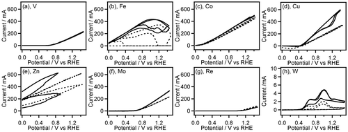
Figure 2. CVs (three-cycle scan) of Ti (a,b), Zr (c,d), Nb (e,f), Ta (g,h), and Ni (i,j) recorded in 0.1 M GC+0.5 M Na₂SO₄ (solid line) and 0.5 M Na₂SO₄ (broken line). The first (a,c,e,g,i) and the second, third (b,d,f,h,j) scan cycles of CVs are depicted separately. The current range of graphs (a–h) is fixed to –20 to 140 μA.

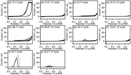
Figure 3. CVs (two-cycle scan) of Ag (a), Pd (b), Pt (c), Au (d), Rh (e,f), and Ir (g,h) recorded in 0.1 M GC+0.5 M Na₂SO₄ (solid line) and 0.5 M Na₂SO₄ (broken line). The current range of graphs (b–e,g) is fixed to –80 to 700 mA.

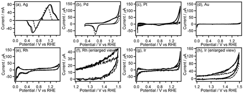
Figure 4. The colors of electrolyte solution after the CV measurements of Fe (a), Co (b), and Cu (c) electrodes in 0.1 M GC+0.5 M Na₂SO₄ (i) and 0.5 M Na₂SO₄ (ii).

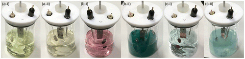
Figure 5. CVs of Pt/C in 0.5 M GC+0.5 M Na₂SO₄ (a) and 0.5 M GC+20 wt% KOH (b) at 50 °C. And CA curves of Pt/C in 0.5 M GC+0.5 M Na₂SO₄ (c) and 0.5 M GC+20 wt% KOH (d) at 50 °C.

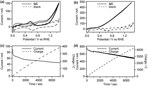
Figure 6. Faradaic yields for CO₂, OX, GO, and HCOOH in GC electro-oxidation (a) at 1.5 V in 0.5 M GC and 0.5 M Na₂SO₄ at 50 °C, (b) at 1.5 V in 0.5 M GC and 20 wt%, i.e. 3.56 M KOH at 50 °C, (c) at 1.2 V in 0.5 M GC and 20 wt% KOH at 50 °C, (d) at 1.5 V in 0.5 M GC and 20 wt% KOH at 40 °C and (e) at 1.5 V in 0.5 M GC and 3.56 M LiOH at 50 °C.

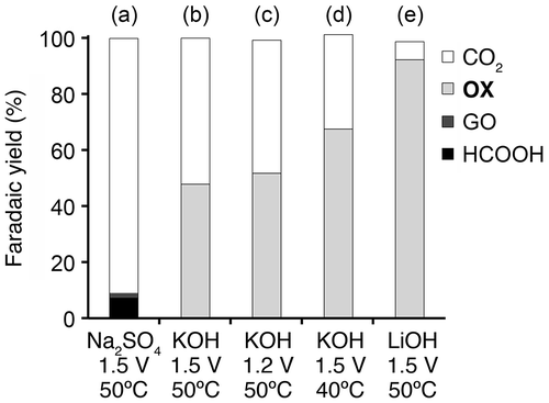
Figure 7. RDE linear sweep voltammograms of TiO₂ in aqueous solution of 0.2 M Na₂SO₄ in the presence and absence of OX with various rotating rates at 50 °C.

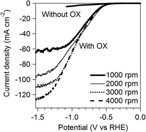
Figure 8. Koutecky–Levich plots at different potentials.

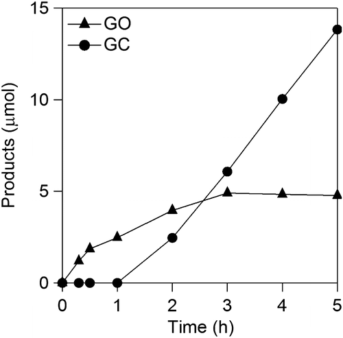
Figure 9. Time courses of GO and GC formations in a CA experiment at −1.5 V vs. RHE using RDE.

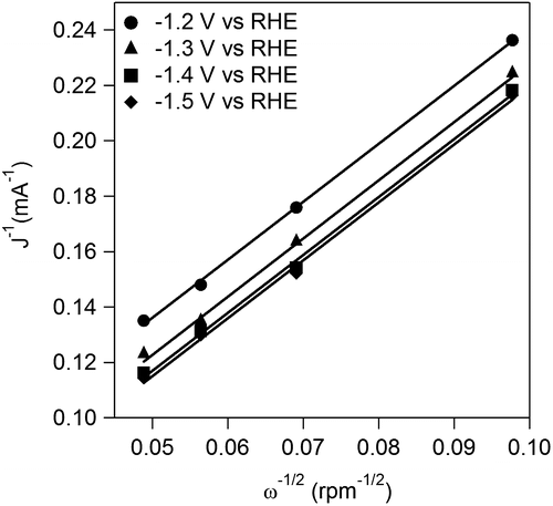
Figure 10a. Yields for GO and GC against specific surface area of TiO₂.

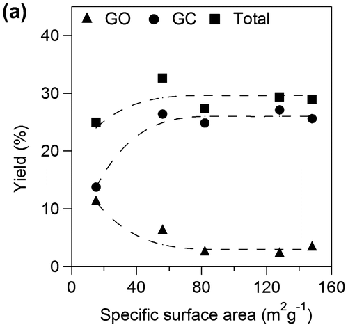
Figure 10b. Faradaic yields for GO and GC against specific surface area of TiO₂.

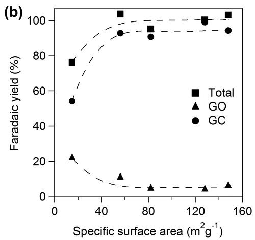
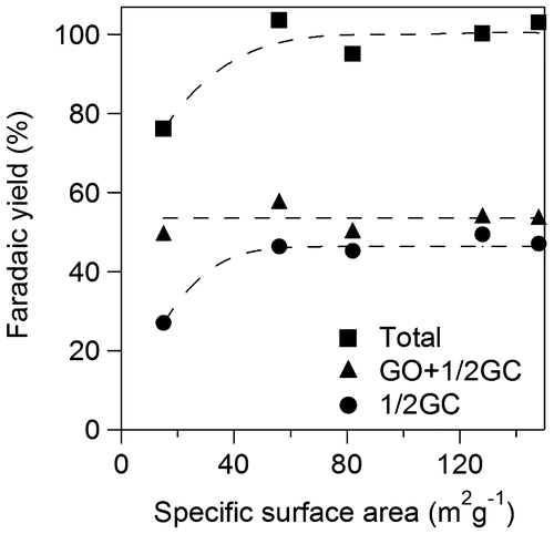
Figure 11. Faradaic yields for GO+1/2GC and 1/2GC against specific surface area of TiO₂.

Scheme 1. Proposed pathway for GC oxidation.