A general representation scheme for crystalline solids based on Voronoi-tessellation real feature values and atomic property data

Figures & data

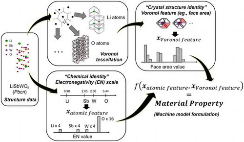
Figure 1. Example of feature binning procedure for (a) electronegativity and (b) Voronoi feature face area (in red) in Pbcn LiSbWO₆ with 4 Li, 4 Sb, 4 W, and 16 O atoms in the unit cell.

Note: Central atom for the Voronoi cell in (b) is shown in magenta.

Table 1. Applied smoothing parameters for various histograms.

Feature	Symbol	Histogram range	Number of bins	Smoothing factor
Electronegativity	EN	0 < EN < 5	50	2
#Voronoi cell edges*	a	0 < v < 70	40	4
Area per Voronoi cell face*	f	0 < e < 90	50	4
#edges per Voronoi cell face*	g	0 < f < 50	30	4
#Voronoi cell faces*	s	0 < a < 15	18	1
Voronoi cell volume*	v	0 < b < 20	20	1
#Voronoi cell vertices*	w	0 < V < 25	25	1
RDF	RDF	0 < RDF < 6 Å	20	0.2 Å

^* Features extracted around each central atom in a unit cell.

Figure 2. (a) Schematic workflow for the extraction procedure implemented for Voronoi tessellation of crystal structures, (b) Test case crystal structure Pbcn LiSbWO₆ (green spheres are Li atoms, brown spheres are Sb atoms, magenta spheres are W atoms, and red spheres are O atoms). Voronoi tessellation for LiSbWO₆ (c) with all atoms considered (1st nearest-neighbor (NN) information), (d) with Li atoms only (2NN information), and (e) with O atoms only (2NN information).

Note: Voronoi atom centers and Voronoi edges are shown in black and gray, respectively.

Table 2. Fitting conditions employed for GBR and SVR models.

Model	Hyperparameter	Condition
GBR	Base tree depth	3
	#Splitting per node	2
	#Base trees, n trees *	n trees ∊ [10, 420]
	#Subsample features for node splitting	$\sqrt{h_{\text{total}}}$, where $h_{\text{total}}$ is the total number of bin features
	#Subsample training data	0.8
	Learning rate	0.1
SVR	Kernel	RBF
	Kernel coefficient	$1/h_{\text{total}}$
	f flatness – deviation tolerance tradeoff, C *	$C\in \left[1000,4000\right],\mathrm{\Delta }C=100$
	Deviation cutoff, $\epsilon$ *	$\epsilon \in \left[0.01,6.0\right],\mathrm{\Delta }\epsilon =0.01$

* Hyperparameters optimized by exhaustive cross-validated search over specified range of parameters.

Figure 3. Test data-set grand average errors for DFT-CE and DFT-BG by (a), (c) GBR (total: 420 trees/data split × 100 data splits = 4200 fitting instances for CE and BG, respectively) and (b), (d) SVR fitting. Test data-set error surface with respect to hyperparameter combination (C and $\epsilon$) for SVR fitting for (c) DFT-CE and (d) DFT-BG; a total of 18,600 regularly-spaced hyperparameter coordinate sets (or fitting instances) each, respectively.

Figure 4. Fitting quality of final models: (a) CE with GBR, (b) CE with SVR, (c) BG with GBR, and (d) BG with SVR. Insets in (a) and (c) show deviance (error residuals) plots terminating at the optimal number of base tree learners for GBR fitting (50 trees for CE and 70 trees for BG, respectively). Optimal hyperparameters (C and $\epsilon$) for SVR fitting are indicated in (b) and (d).

Table 3. Comparison of predictive accuracy between EN+VORO and RDF-based final machine models with ICSD-based DFT calculated data-set (140 compounds).

Target property	Feature vector	Model	Test set RMSE	Test set MAE
DFT-CE (eV/atom)	EN+VORO	GBR	0.316	0.258
		SVR	0.247	0.196
	RDF	GBR	0.337	0.281
		SVR	0.266	0.202
DFT-BG (eV)	EN+VORO	GBR	0.722	0.587
		SVR	0.497	0.387
	RDF	GBR	0.558	0.433
		SVR	0.408	0.329

Figure 5. Test data-set grand average errors (from 100 random data splitting) for (a) DFT-CE, (c) DFT density (DFT-d), (e) DFT-BG, and (g) DFT decomposition energy (DFT-Ed) by GBR fitting. Final models have (b) 120, (d) 160, (f) 300, (h) 430 trees, respectively.

Notes: Data-sets are comprised with 1000 Li-containing oxides taken from Materials Project (see Table S2 of Supporting Information for the materials ID list) [1].

Table 4. Comparison of predictive accuracy between EN+VORO- and RDF-based final machine models using Materials Project data-set (1000 compounds).

Target property	Feature vector	Model	RMSEtest	MAEtest
DFT-CE (eV/atom)	EN+VORO	GBR	0.210	0.155
		SVR	0.274	0.196
	RDF	GBR	0.381	0.284
		SVR	0.410	0.318
DFT-d (g/cm^3)	EN+VORO	GBR	0.575	0.436
		SVR	0.532	0.404
	RDF	GBR	0.653	0.479
		SVR	0.603	0.444
DFT-BG (eV)	EN+VORO	GBR	0.661	0.515
		SVR	0.668	0.541
	RDF	GBR	0.728	0.579
		SVR	0.730	0.590
DFT-Ed (meV/atom)	EN+VORO	GBR	26.0	22.0
		SVR	31.0	26.0
	RDF	GBR	27.0	21.0
		SVR	30.0	25.0

Figure 6. Scaled variable importance (VI) plot of bin features from the final GBR models for (a) DFT-CE and (b) DFT-BG.

Notes: Horizontal axis denotes bin index number of increasing real value feature from left to right. Vertical axis shows the labels of the subset histogram features (see Table 1 for description). VI scores are scaled to 100 while colorbar maximum is set only to 50 to enhance visual distinction among features.

Figure 7. (a) Average number of vertices vs. counted average face area <0.2 from Voronoi tessellations of atom centers, (b) histogram for face areas relative to average per Voronoi cell for Pbcn LiSbWO₆ crystal structure.

Jain A , Hautier G , Moore CJ , et al . A high-throughput infrastructure for density functional theory calculations. Comp Mater Sci. 2011;50:2295–2310.10.1016/j.commatsci.2011.02.023

 Web of Science ®Google Scholar