Microstructural characterization and properties of selective laser melted maraging steel with different build directions

Figures & data

Figure 1. Effect of volumetric laser energy (E_v ) on the relative density of SLM-produced MS.

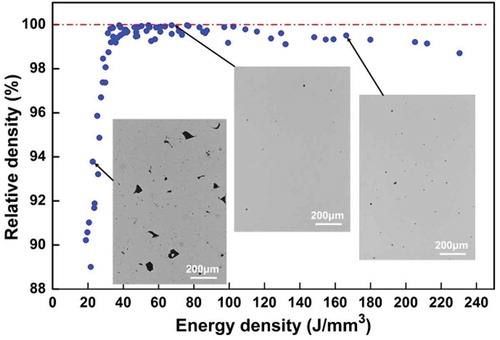
Figure 2. DSC trace of the as-fabricated MS by SLM.

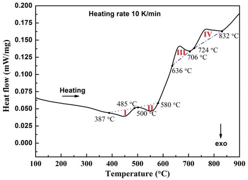
Figure 3. Representative OM and SEM images taken from the horizontal (a)–(c) and vertical (d)–(f) cross-sections of the AF specimen.

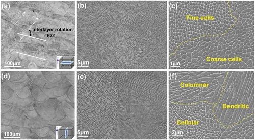
Figure 4. EBSD analysis of the vertical cross-sections taken from the as-fabricated specimen: (a) color inverse pole figure (IPF) showing grain orientation distributions and (b) corresponding pole figure (PF), (c) grain size distribution, (d) high-magnification IPF and (e) grain boundary map.

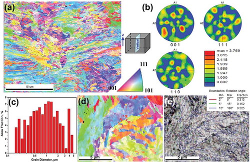
Figure 5. TEM images of AF specimen: (a) BF-TEM image taken from the horizontal cross-section showing cellular structures, (b) zoom-in image of (a) showing high-density dislocations, and (c) BF-TEM image with corresponding SAED taken from the vertical cross-section exhibiting acicular martensites.

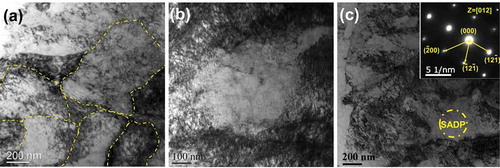
Figure 6. TEM analysis of precipitate characteristics in age-treated specimen: (a) BF-TEM overview showing massive nanoprecipitates embedded in amorphous matrix, (b) zoom-in BF-TEM image of (a) showing precipitate morphology, (c) zoom-in image taken from the given region of (b), (d) high-resolution TEM (HRTEM) image showing the coherent interface with elastic strain; and (e) HRTEM image showing the complete coherent interface.

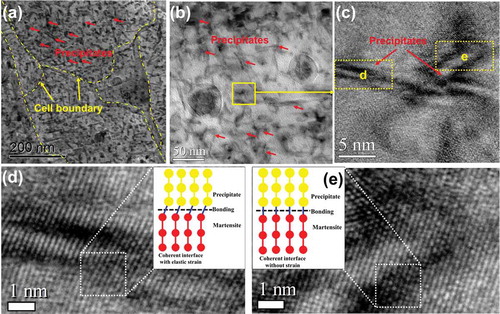
Figure 7. Residual stress measured from the horizontal surface of (a) AF and (b) AT specimens.

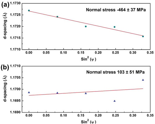
Table 1. Comparison of the mechanical properties for grade 300 MS fabricated by SLM and conventional wrought method.

Building orientation	Specimens	UTS (MPa)	YS (MPa)	El (%)	HRC
Horizontal	SLM as-fabricated	1165 ± 7	915 ± 7	12.4 ± 0.1	34.8 ± 0.2
	SLM aged	2014 ± 9	1967 ± 11	3.3 ± 0.1	54.6 ± 0.8
	SLM solution	1025 ± 5	962 ± 6	14.4 ± 0.4	29.8 ± 1.3
	SLM solution-aged	1943 ± 8	1882 ± 14	5.6 ± 0.1	53.5 ± 0.8
Vertical	SLM as-fabricated	1085 ± 19	920 ± 24	11.3 ± 0.3	35.7 ± 1.1
	SLM aged	1942 ± 31	1867 ± 22	2.8 ± 0.1	52.9 ± 1.2
	SLM solution	983 ± 13	923 ± 16	13.7 ± 0.7	27.5 ± 0.4
	SLM solution-aged	1898 ± 33	1818 ± 27	4.8 ± 0.2	51.3 ± 0.9
Standard	Wrought ^[Citation38]	1000–1170	760–895	6–15	35
	Wrought aged ^[Citation3,Citation33]	1930–2050	1862–2000	5–7	52

Figure 8. Impact energies (a) and fracture morphologies (b) of as-fabricated and heat-treated MS specimens with horizontal and vertical building directions.

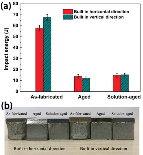
Table 2. Tribological properties of SLM fabricated MS specimens.

Specimens	Coefficient (μ)	Depth (μm)	Width (μm)	A (μm^2)	Kc (mm^3/Nm)
As-fabricated	0.62	7.74	783	4428	4.43 × 10^−8
Aged	0.56	2.98	663	1912	1.91 × 10^−8
Solution-aged	0.58	4.16	706	2526	2.53 × 10^−8

Figure 9. Friction coefficient (a), 3D wear track morphology (b), and sectional line profiles of wear track of SLM specimens.

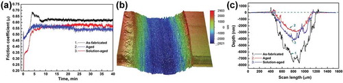
Figure 10. SEM micrographs of as-fabricated and heat-treated MS specimens after wear tests.

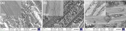
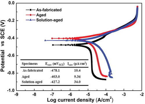
Figure 11. Potentiodynamic polarization curves and summarized relative corrosion properties of as-fabricated and heat-treated MS specimens.

Kempen K , Yasa E , Thijs L , et al. Microstructure and mechanical properties of selective laser melted 18Ni-300 steel. Physics Procedia. 2011;12:255–263.

 Google Scholar

A.I.H. Committee . Properties and selection: irons steels and high performance alloys. In: ASM handbook. USA: Materials Information Company; 1991. p. 1872–1873.

 Google Scholar

S.A. 6514H . Steel, maraging, bars, forgings, tubing, and rings 18.5Ni - 9.0Co - 4.9Mo - 0.65Ti - 0.10Al consumable electrode vacuum melted, annealed. USA: SAE International; 2012. p. 8.

 Google Scholar