Solution based freeze cast polymer derived ceramics for isothermal wicking - relationship between pore structure and imbibition

Figures & data

Figure 1. Process scheme of monolith preparation by solution-based freeze casting of polymeric solutions.

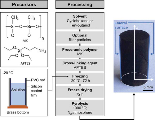
Table 1. Labeling and composition of studied samples.

		Solid loading	Filler loading	Condition of sample^1
Sample labeling	Solvent	wt%	vol%	XXX
CH20/0_XXX	Cyclohexane	20	0	EC/EO/N
CH40/0_XXX	Cyclohexane	40	0	EC/EO/N
TBA40/0_XXX	Tert-butyl alcohol	40	0	EC/EO/N
CH40/50_XXX	Cyclohexane	40	50	EC/EO/N

¹EC = experimental closed; EO = experimental open, N = numerical results.

Table 2. Liquid properties of HFE-7500 and water at 298.15 K and 101,325 Pa. Source: Product data sheet of supplier 3M.

	Surface tension σ 10^−3	Density ρ	Dynamic viscosity μ 10^−3
Liquid	N m^−1	kg m^−3	Pa s
HFE-7500	16.2	1614	1.24
Water	–	998	1.00

Figure 2. Schematic representation of the experimental wicking device.

Table 3. Geometrical characteristics and macroscopic parameters of the investigated samples.

	H	D		Rmerc	KWicking	KDarcy	j(EC)	j(EO)	heq	meq
	10^−3 m	10^−3 m	ϕ	10^−6 m	10^−14 m^2	10^−14 m^2	10^−4 kg s^−1 m^−2	10^−4 kg s^−1 m^−2	m	kg
CH20/0	32.9 ± 0.1	13.7 ± 0.1	0.793 ± 0.003	10.5 ± 0.6	48.4 ± 3.2	6.43 ± 1.07	3.88 ± 0.10	24.3 ± 3.10	0.195	0.037
CH40/0	25.9 ± 0.1	13.6 ± 0.2	0.608 ± 0.023	7.0 ± 0.5	3.9 ± 0.8	0.10 ± 0.04	0.33 ± 0.01	1.22 ± 0.04	0.292	0.041
TBA40/0	22.9 ± 0.1	14.7 ± 0.1	0.635 ± 0.003	5.5 ± 0.1	9.8 ± 1.3	1.31 ± 0.73	1.29 ± 0.06	8.82 ± 0.68	0.372	0.064
CH40/50	25.2 ± 0.2	14.6 ± 0.1	0.631 ± 0.002	5.5 ± 0.2	12.9 ± 0.6	3.98 ± 0.44	1.47 ± 0.18	4.02 ± 0.17	0.372	0.063

Figure 3. Characteristic cross-sectional SEM images of the pore structure of pyrolyzed monoliths and simplified schemes of the pore structure for (a) CH20/0, (b) CH40/0, (c) TBA40/0 and (d) CH40/50; SEM images of the lateral surface of sample CH40/0 (e) as prepared (to a great extend closed) and (f) after removing the dense layer (open lateral surface).

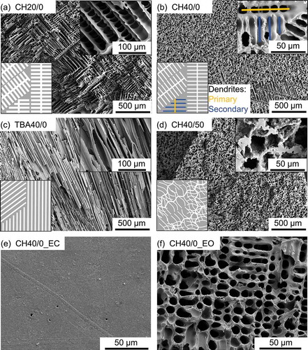
Figure 4. Open porosity ϕ and mean pore window diameter 2Rmerc for all studied samples obtained by mercury intrusion.

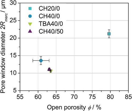
Figure 5. Water flux through the lateral surface j obtained by constant head permeability measurements for all studied samples as prepared and after removing the dense outside layer.

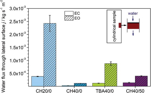
Figure 6. The squared height over time for the investigated samples. Equation (3)(3) $\frac{m^2}{t}=\frac{4\sigma cos\theta {\rho }_l^2{A}^2\varphi }{{\mu }_l}\frac{K}{R_s}.$(3) was fitted to the experimental line.

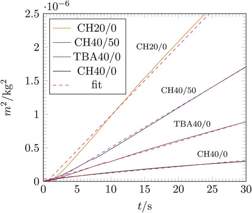
Figure 7. Wicking results of the samples with a lateral open and lateral closed surface compared with the calculated wicking results of Equation (5)(5) $\frac{2\sigma cos\theta }{R_s}=\frac{\varphi {\mu }_l\dot{h}h}{K}+{\rho }_{l}gh.$(5) ; The grey areas represent the deviation of the calculation caused by the measurement error of the macroscopic parameters.

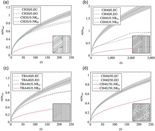
Figure 8. Wicking curves for all investigated pore morphologies of samples with open lateral surface.

Table 4. Scaled parameters of Equation (8)(8) $1=b\dot{h}h+ch.$(8) describing wicking.

	b	c
	10^5 s m^−2	m^−1
CH20/0	6.6	5.13
CH40/0	41.8	3.42
TBA40/0	13.6	2.69
CH40/50	10.3	2.69