Development of spectral decomposition based on Bayesian information criterion with estimation of confidence interval

Figures & data

Figure 1. Three examples of artificially measured spectra with Gaussian noise. The solid line is the true curve $f\left(x;{\theta }^{\ast }\right)$ and the dots are the artificially measured spectral data: (a) $\mathrm{S}/\mathrm{N}=20.0$ and $\mathrm{\Delta }=0.5$, (b) $\mathrm{S}/\mathrm{N}=20.0$ and $\mathrm{\Delta }=0.1$, and (c) $\mathrm{S}/\mathrm{N}=0.2$ and $\mathrm{\Delta }=0.5$.

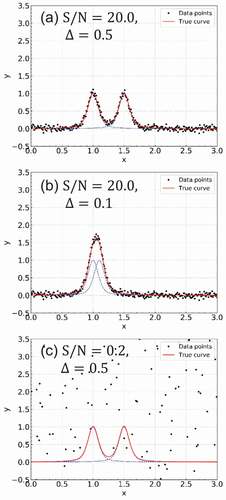
Table 1. Settings of the inverse temperature ${\left\{{\beta }_m\right\}}_{m=1}^M$ corresponding to Eq. (18).

$\sigma$	0.0005	0.001	0.002	0.005	0.01	0.02	0.05	0.1	0.2	0.5	1	2	5	10
S/N	2000	1000	500	200	100	50	20	10	5	2	1	0.5	0.2	0.1
$\gamma$	1.2	1.5	1.5	1.5	1.5	1.5	1.5	1.5	1.5	1.5	1.5	1.5	1.5	1.5
$M$	128	64	64	64	44	44	32	32	32	32	32	32	32	32

Figure 2. (a)–(c) Results of model selection by Bayesian estimation respectively corresponding to spectral data in Figure 1(a)–(c).

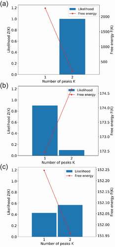
Figure 3. Results of model selection for various peak-to-peak distances $\mathrm{\Delta }$ and S/N ratios. The values in the figure indicate the posterior probability $p\left(K=2|D\right)$ for $K=2$.

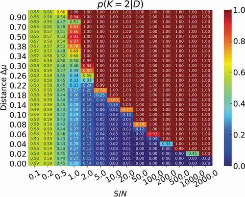
Figure 4. Posterior distribution of each parameter when Bayesian estimation is performed on the spectral data in Figure 1(a). Dashed lines indicate the true parameter values used to generate the spectral data.

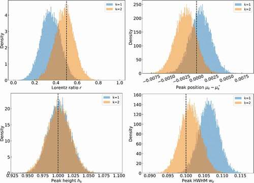
Figure 5. STD of the posterior distribution as a function of the S/N ratio for Δ = 0.5. Triangles and inverted triangles are respectively the STDs of the parameters for the first and second peaks.

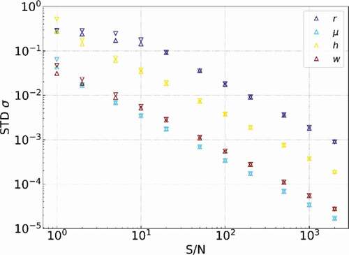
Figure 6. STD as a function of the peak-to-peak distance $\mathrm{\Delta }$ for S/N = 100.0. Triangles and inverted triangles are respectively the STDs of the parameters for the first and second peaks.

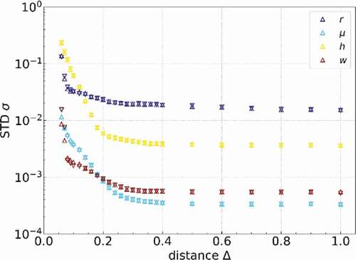
Table 2. Values of the fitted parameters 2$\left\{B_j,C_j,D_j,E_j\right\}$ in Eq. (19).

Parameter	Bj	μj	Dj (fixed)	Ej
r	1.708	−4.626	2.5	−1.394
μ	0.324	−3.271	2.5	−0.216
h	0.355	−5.756	2.5	−0.540
w	0.504	−3.158	2.5	−0.760

Figure 7. Schematic diagrams of values obtained using Eq. (19)(A-19) $s\left(\mathrm{\Delta },\frac{\sigma }{h_0}\right)=\frac{\sigma }{h_0}B\left\{{\left(\frac{\mathrm{\Delta }-E}{D}\right)}^C+1\right\}$(A-19) . (a) Scaled STD $\tilde{s}$ as a function of S/N $\left(=h_0/\sigma \right)$ for $B=10.0,1.0,0.1$ and $0.01$, where the peak-to-peak distance $\mathrm{\Delta }$ is sufficiently large: $\mathrm{\Delta }=10.0,\hspace{0.17em}C=-3.0,\hspace{0.17em}D=2.0$ and $E=0.0$. (b) $\tilde{s}$ as a function of the peak-to-peak distance $\mathrm{\Delta }$ for several conditions of $\left\{C,D,E\right\}$ when we set the prefactor of Eq. (19(A-19) $s\left(\mathrm{\Delta },\frac{\sigma }{h_0}\right)=\frac{\sigma }{h_0}B\left\{{\left(\frac{\mathrm{\Delta }-E}{D}\right)}^C+1\right\}$(A-19) ) $\sigma B/h_0=1$.

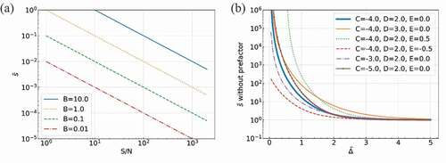
Figure 8. Results of regression using the fitting function in Eq. (19)(A-19) $s\left(\mathrm{\Delta },\frac{\sigma }{h_0}\right)=\frac{\sigma }{h_0}B\left\{{\left(\frac{\mathrm{\Delta }-E}{D}\right)}^C+1\right\}$(A-19) of the STDs of the posterior distributions for each parameter. Parameters are the (a) Lorentz–Gauss mixing ratio $r_k$, (b) peak position ${\mu }_k$, (c) peak height $h_k$, and (d) HWHMs of the peaks $w_k$.

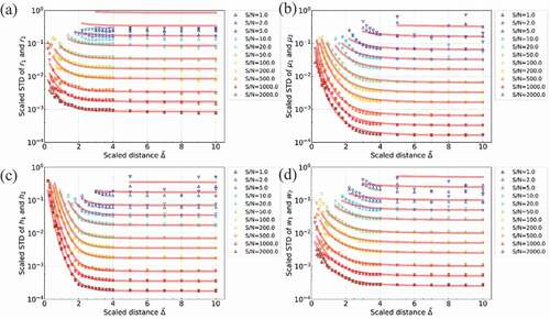
Figure 9. Fitted spectra from Bayesian estimation (a) and BIC-fitting (b) for the experimental valence spectrum of SiO₂. Open circles are the experimental spectrum, the orange line is the fitted spectrum, the green line is the background, and the black lines are all peaks above the background.

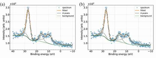
Figure 10. Results of model selection through Bayesian estimation (a) and BIC-fitting (b) for the experimental valence spectrum of SiO₂. The red circle in (b) indicates the model with the minimum BIC.

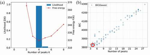
Figure 11. Two-dimensional histogram of PC1 and PC2 obtained by PCA of EMC sampling.

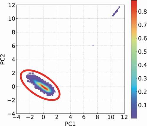
Table 3. Calculated confidence intervals of the posterior distribution for all peak parameters and those estimated using Eq. (19).

Parameter	Confidence interval for peak k = 1	Confidence interval for peak k = 2	Confidence interval estimated using Eq. (19) and the BIC-fitting model
$\mu$	0.22	0.21	0.34
$h$	2.35	3.69	5.48
$w$	0.33	0.32	0.40
$r$	0.12	0.27	$-$

Figure 12. Posterior probability densities of peak parameters $\left\{{\mu }_k,h_k,w_k,r_k\right\}\left(k=1,2\right)$ for two peaks located at about $E_B=10$ and $16$ eV for the valence spectrum of SiO_2.

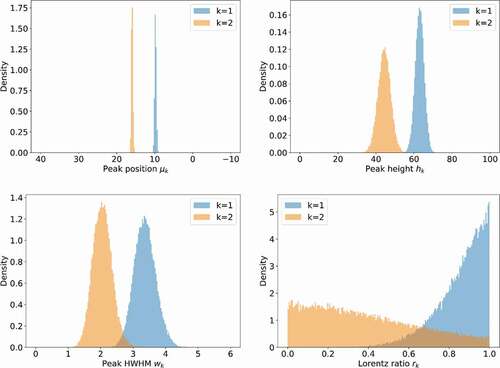
Figure A-1. Results of model selection and posterior distributions $p\left(w_k|D,K\right)$ and $p\left(r_k|D,K\right)$. (a)–(e) only differ in the initial random seeds used in generating the spectral data sets under the same conditions as those in Figure 1(a).

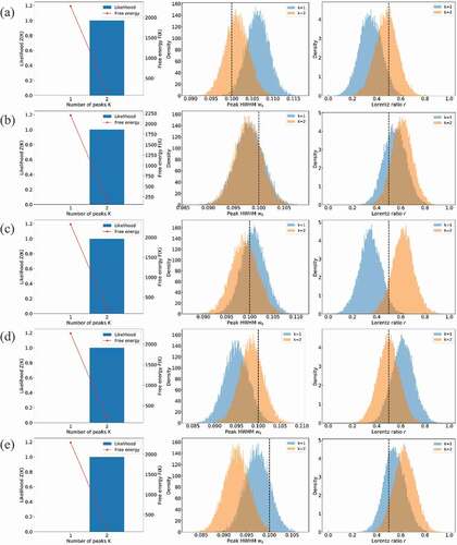
Figure A-2. Two-dimensional distribution of parameters $\theta$. The diagonal components of the figure show the histogram of the posterior distribution of each parameter. The lower off-diagonal components are two-dimensional distributions, whereas the upper off-diagonal components show the coefficients of correlation between two parameters. The dotted lines indicate the true parameter values used to generate the spectral data.

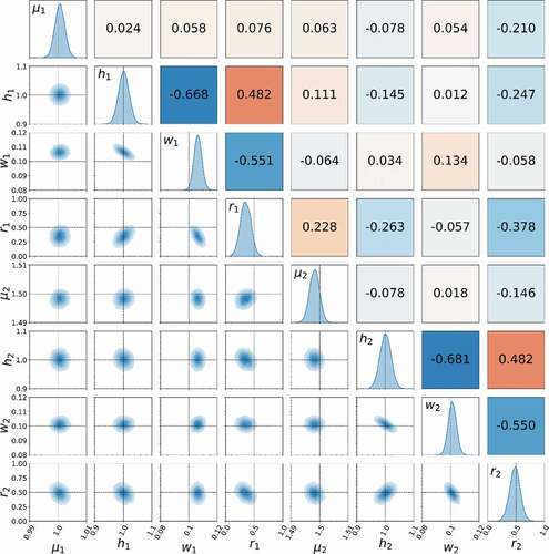
Figure E-1. Two examples of artificial spectra that have two peaks with different heights: (a) $h_1^{\ast }=1.0,h_2^{\ast }=0.5$, (b) $h_1^{\ast }=1.0,h_2^{\ast }=0.1$. The other parameters are the same. Open circles are the artificial spectrum, the orange line is the fitted spectrum, and the black lines are the peak components.

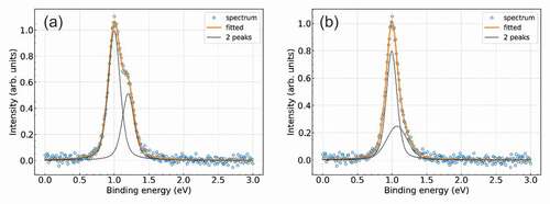
Figure E-2. Posterior distribution of each parameter when Bayesian estimation is performed on the spectral data in Fig. E-1(a). The dashed lines indicate the true parameter values used to generate the spectral data.

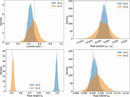
Figure E-3. Posterior distribution of each parameter when Bayesian estimation is performed on the spectral data in Fig. E-1(b). The dashed lines indicate the true parameter values used to generate the spectral data.

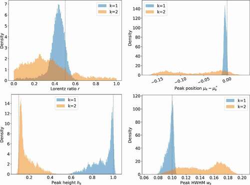
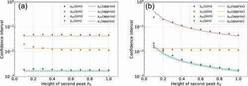
Figure E-4. Confidence intervals of peak parameters as a function of the height of the second peak $h_2$ for peaks 1 (a) and 2 (b). (sim) indicates values simulated by the Bayesian EMC method, (approx) indicates values calculated with the approximated formula (19).