Finite element analysis of the fracture statistics of self-healing ceramics

Figures & data

Figure 1. Schematic response characteristics of damage-healing processes by the damage-healing constitutive model under uniaxial tensile conditions: (a) crack occurrence and healing on a microstructural scale; (b) stress–strain relation; and (c) variation of cracks in an element with an embedded cohesive zone relationship.

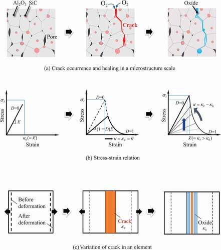
Figure 2. Fracture mechanics model based on an ellipsoidal (spheroidal) pore [35].

Figure 3. FE models of the three-point bending test and healing: (a) non-damaged specimen; (b) as-cracked specimen and the details of initial damaged part.

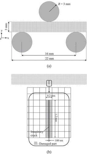
Figure 4. Simulation flow.

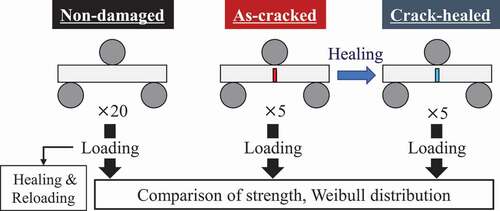
Table 1. Mechanical parameters of Al₂O₃/15 vol% SiC.

E [GPa]	ν	KIC [MPa mm^0.5]	k
398	0.21	120	11.3

Table 2. Parameters for self-healing of Al₂O₃/15 vol% SiC.

Ah [s^−1]	Qh [J/mol]	R [J/(mol/K)]	n	wexp [μm]
1.04 × 10^4	3.87 × 10^5	8.31	0.836	0.1
${\xi }_1,{\xi }_2$	Th [K]	$a_{O_2}$	${\kappa }_s$
5.0	1623	0.21	4750 × 10^−6

Table 3. Microstructure distribution characteristics.

Relative density		Pore size [μm]		Aspect ratio		Grain size [μm]
μρ	σρ	μR	σR	μA	σA	μc	σc
0.99	0.001	0.437	3.18	1.0	0.5	0.6	0.1

Figure 5. Fracture stress distribution in the three specimens, where the colors in the contour map represent the elemental values. Here, specimens (a), (b), and (c) correspond to specimens of minimum, median, and maximum bending strengths, respectively.

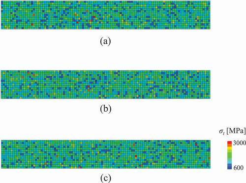
Figure 6. Histogram of the microstructure data of the elements obtained by one specimen: (a) relative density; (b) pore size (major radius); (c) aspect ratio of the pore; and (d) grain size. The vertical axis of the graphs represents the number of elements.

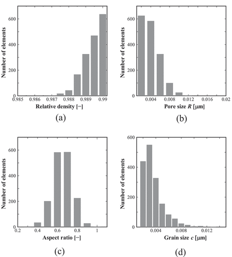
Figure 7. The damage variable distribution in the specimens corresponding to that in Fig. 5. The contour map shows the result of damage propagation in specimens under the three-point bending test. The blue elements represent the state without damage, whereas the red elements represent the damaged state.

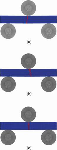
Figure 8. Relationship between the bending stress and deflection obtained by three specimens shown in Fig. 5. The graph includes the result of the as-cracked specimen.

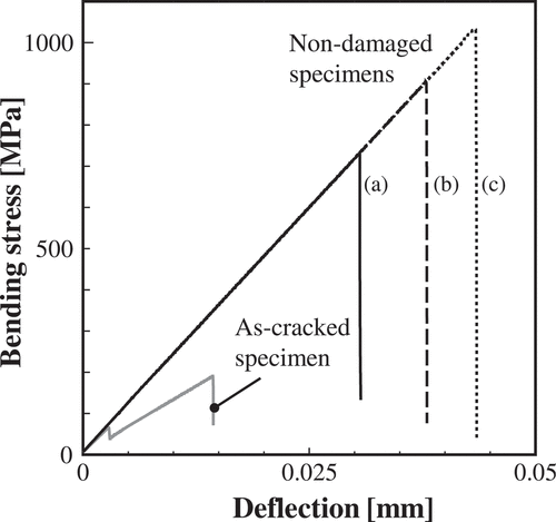
Figure 9. Time series snapshots of the distribution of damage variable D in the specimen of Fig. 5(a) during the healing stage under a prescribed condition after the unloading (temperature T_h = 1623 [K] and oxygen partial pressure $a_{O_2}=0.21$).

Figure 10. FEA results of reloading for completely healed specimen shown in Fig. 9: (a) the contour map of the damage variable: (b) bending stress–deflection relationship. The white frame in the contour map depicts the path of damage progression in the first loading.

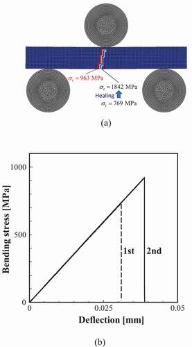
Figure 11. Time series snapshots of the healing process of the initial damaged part in an as-cracked specimen. The blue elements represent the state without damage, whereas the red elements represent the damaged state.

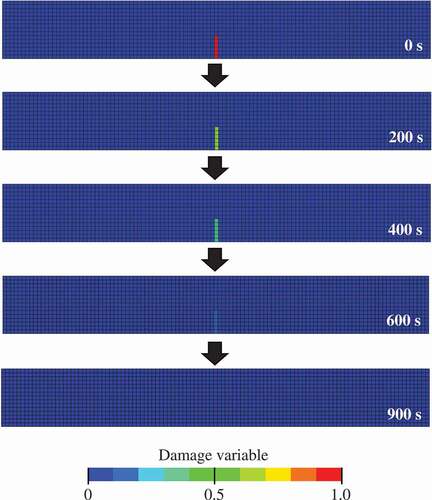
Figure 12. Relationships between bending stress and deflection for as-cracked and crack-healed specimens. The figure also depicts the contour map of the damage variable. The white frame in the contour map depicts the initial damaged part.

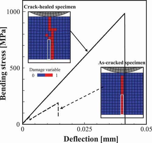
Figure 13. Weibull distributions obtained by the FEA of non-damaged, as-cracked, and crack-healed specimens. The calculated combinations of the Weibull modulus m and the scale parameter β [MPa] are as follows: non-damaged specimen (13.4, 983 [MPa]), as-cracked specimen (4.5, 225 [MPa]), and crack-healed specimen (19.5, 975 [MPa]).

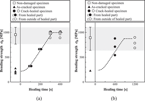
Figure 14. Time dependence of strength recovery obtained by (a) FEA and (b) experiment. The plots correspond to peak values of the bending stress-deflection relationships.

Quinn GD, Morrell R. Design data for engineering ceramics: A review of the flexure test. J Am Ceram Soc. 1991;74(9):2037–2066.

 Web of Science ®Google Scholar