
Figures & data
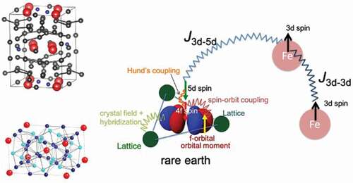
Figure 1. Magnetism in a rare-earth magnet compound.
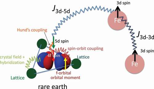
Figure 2. In the coherent potential approximation, random alloy is replaced with an impurity problem.
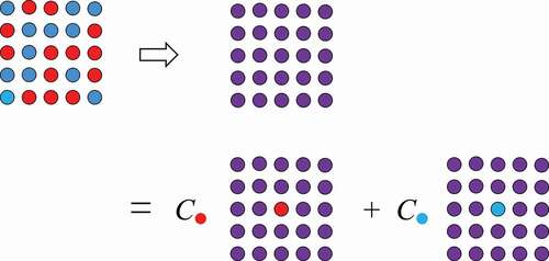
Figure 3. Intersite exchange coupling for the ferromagnetic state and LMD (local moment disorder) state.
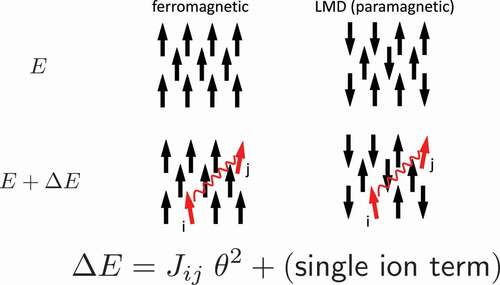
Figure 4. Curie temperatures () of
Fe
B,
Co
B,
Fe
,
Co
and
Fe
Ti.
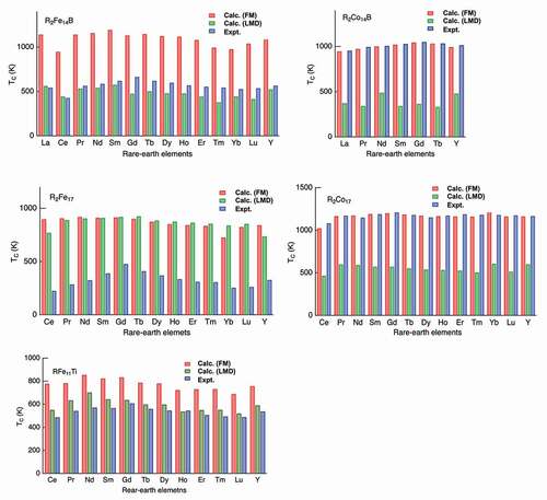
Figure 5. Hierarchical clustering of rare-earth transition-metal compounds by obtained dissimilarity voting machine using experimental Curie temperature data. From Ref [Citation68].
![Figure 5. Hierarchical clustering of rare-earth transition-metal compounds by obtained dissimilarity voting machine using experimental Curie temperature data. From Ref [Citation68].](/cms/asset/0d2c8e82-5177-4585-9b88-d7877c9901dd/tsta_a_1935314_f0005_oc.jpg)
Figure 6. Potentially formable phases of Nd-Fe-B systems obtained by theoretical exploration. See Ref [Citation98]. for the comparison between direct screening by first-principles calculation and virtual screening using machine learning. From Ref [Citation98].
![Figure 6. Potentially formable phases of Nd-Fe-B systems obtained by theoretical exploration. See Ref [Citation98]. for the comparison between direct screening by first-principles calculation and virtual screening using machine learning. From Ref [Citation98].](/cms/asset/1381cff9-6afd-44c9-8a79-2fa39a3a0d39/tsta_a_1935314_f0006_oc.jpg)
Figure 7. Schematic of Bayesian optimization. Already sampled points are shown by closed circles. In the Bayesian optimization, the next candidate is selected by taking account of the uncertainty of a model (shaded area) in addition to the mean value (solid line) of a prediction model obtained by the sampled data. From Ref [Citation100].
![Figure 7. Schematic of Bayesian optimization. Already sampled points are shown by closed circles. In the Bayesian optimization, the next candidate is selected by taking account of the uncertainty of a model (shaded area) in addition to the mean value (solid line) of a prediction model obtained by the sampled data. From Ref [Citation100].](/cms/asset/d292184f-49e8-495b-a75d-27c6dbae4ecb/tsta_a_1935314_f0007_b.gif)
Figure 8. Schematic illustration of data-assimilation method.
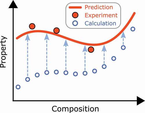
Figure 9. Magnetization of (NdCe
)
(Fe
Co
)
B at 0 K and at 400 K. At 0 K, the magnetization is the highest at (
) = (0,0), and monotonically decreases with increasing
and
. At 400 K, the magnetization increases with increasing Co concentration for small
, and turns to decrease for further increasing
. From Ref [Citation101].
![Figure 9. Magnetization of (Nd 1−γCe γ) 2(Fe 1−δCo δ) 14B at 0 K and at 400 K. At 0 K, the magnetization is the highest at (δ,γ) = (0,0), and monotonically decreases with increasing δ and γ. At 400 K, the magnetization increases with increasing Co concentration for small δ, and turns to decrease for further increasing δ. From Ref [Citation101].](/cms/asset/e3a94327-7a70-463e-b434-b026533cadbf/tsta_a_1935314_f0009_oc.jpg)
Table 1. The inner coordinates for Nd2Fe14B [Citation70]
Table 2. The inner coordinates for Sm2Fe17 [Citation77]
Table 3. The inner coordinates for Sm2Fe17N3.
Table 4. The inner coordinates for SmFe12 [Citation75]