Formation and thermal stability of two-phase microstructures in Al-containing refractory compositionally complex alloys

Figures & data

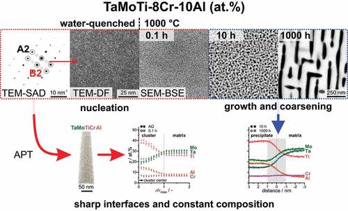
Figure 1. SEM-BSE micrographs of: (a) as-cast (AC); (b) as-homogenized (AH) condition after heat treatment at 1600°C for 20 h with cooling inside the furnace with 100 K/h; (c) as-quenched (AQ); subsequent to the AH condition, the samples were annealed at 1200°C for 0.5 h, followed by quenching in water.

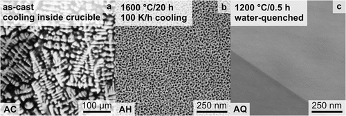
Table 1. Determined chemical composition ${\bar{x}}_{\mathit{i}}$ of the AH condition by means of inductively coupled plasma-optical emission spectrometry (ICP-OES), presented in at.%. The O and N concentrations by hot gas extraction are given in wt.-ppm.

	${\bar{x}}_{\mathit{i}}$ / at.%					Impurities / wt.-ppm
Desired composition / at.%	Ta	Mo	Ti	Cr	Al	O	N
27.3Ta-27.3Mo-27.3Ti-8Cr-10Al	28.1	28.3	27.7	7.2	8.7	92 ± 23	45 ± 11

Figure 2. TEM and APT investigations of the AQ condition. (a) TEM-SAD pattern acquired close to the [011] zone axis (ZA). Selected spots are labeled, B2 superlattice spots are labeled in red and A2 fundamental spots are labeled in black. (b) TEM-DF micrograph taken with the objective aperture on a $⟨100⟩$ spot (B2 superlattice). (c) Reconstruction presenting the elemental distribution within the examined tips; 0.5% of all detected and assigned ions displayed.

Figure 3. Evaluation of one representative APT tip in the AQ condition. (a) Frequency distribution analysis of each constituent element, the individual ${\mu }_i$ values of which are presented. The binomial distributions are displayed by solid lines, while the experimental distribution is depicted by individual data points (open circles). (b) Cluster concentration profile presented in at.%. The length scale is normalized by the cluster size; therefore, the core of the cluster is at the origin. To exemplify that the difference in APT analysis modes is minor, one data set for laser and one for voltage mode are displayed.

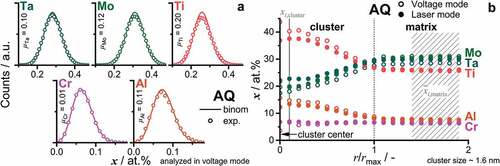
Table 2. Statistical data on ion distribution and chemical composition of clusters. Pearson correlation coefficient ${\mu }_i$ was determined from three APT tips of the AQ condition. Two of the tips were analyzed in laser mode, while one was in voltage mode. Chemical composition $x_i$ (in at.%) at the core of the clusters ($x_{\mathit{i},\mathrm{cluster}}$) and matrix (${\bar{x}}_{\mathit{i},\mathrm{matrix}}$), as determined by APT cluster analysis of the tip investigated in voltage mode.

$\mathit{i}$	Ta	Mo	Ti	Cr	Al
${\mathit{\mu }}_{\mathit{i}}$	0.11 ± 0.02	0.15 ± 0.03	0.21 ± 0.01	0.03 ± 0.02	0.13 ± 0.02
${\bar{\mathit{x}}}_{\mathit{i},\mathbf{matrix}}$	28.5 ± 0.1	31.0 ± 0.1	25.9 ± 0.1	6.6 ± 0.1	7.7 ± 0.1
${\mathit{x}}_{\mathit{i},\mathbf{cluster}}$	18.1	19.9	40.3	6.9	14.7

Figure 4. SEM-BSE micrographs with primarily $\mathit{Z}$ contrast taken within a single grain after heat treatment of: (a) 1000°C/0.1 h; (b) 1000°C/1 h; (c) 900°C/0.1 h, with higher magnification inset; (d) 900°C/1 h; (e) 800°C/0.1 h; (f) 800°C/1 h. The same magnification is used for all micrographs, except the inset in (c).

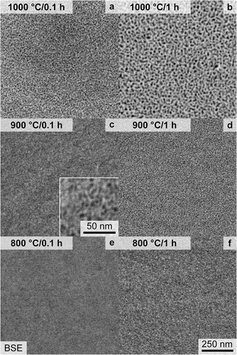
Figure 5. Concentration profiles of the constituent elements over the precipitate/matrix boundary. (a) AQ and 0.1 h, by cluster analysis. AQ data is the same as displayed in Figure 3b. The cluster center is located at r/r_max = 0 and the boundary at one unit of normalized radius. (b) 10 h and 1000 h were evaluated by means of proximity histograms of iso-concentration surfaces with x_Ti + x_Al = 47 at.%. (c) Determined concentration in the matrix (left) and precipitates (right) for AQ and 1000°C/0.1 h, 10 h and 1000 h. Error bars smaller than the symbol size are omitted.

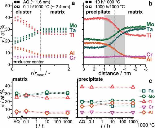
Figure 6. SEM-BSE micrographs with primarily Z contrast taken within single grains after a heat treatment of: (a, b, c) 1000°C, (d, e, f) 900°C and (g, h, i) 800°C as well as (a, d, g) 10 h, (b, e, h) 100 h and (c, f, i) 1000 h. The same magnification is used for all micrographs.

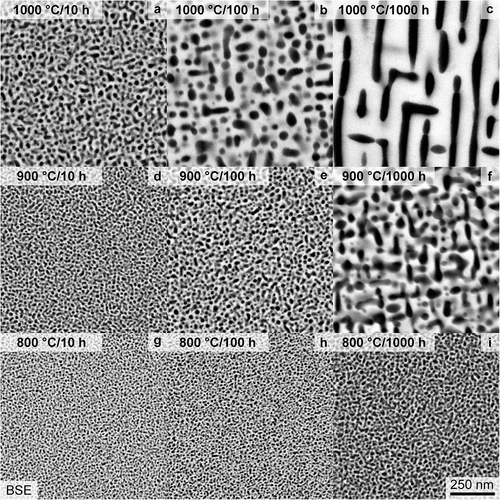
Figure 7. Evaluation of the SEM micrographs based on binarization and morphological operations to separate the two phases. (a) Mean diameter of the particles, $d_{\mathrm{mean}}$, as a function of the cube root annealing time, $t^{1/3}$. (b) Inter-particle spacing between the precipitates. (c) Area fraction of the precipitates, $\mathit{f}$. Schematic differentiation between the growth and coarsening/ripening phase is displayed. The same symbols and colors for each temperature are used throughout this figure.

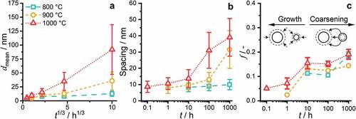
Figure 8. TEM investigations on a selected grain boundary (vertical in the figure) after 1000°C/1000 h; (a) HAADF micrograph of the grain boundary. A hole in the FIB-prepared thin foil is marked with ‘x’. (b) EDS Mappings corresponding to the HAADF micrograph in (a) of the same field of view. The Laves phase is marked with white arrows.

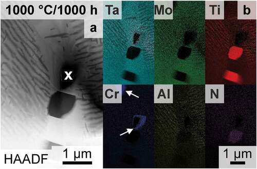
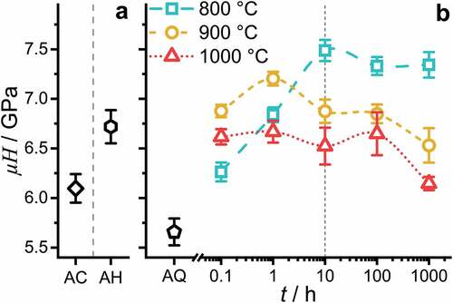
Figure 9. Hardness $\mathit{\mu H}$ evaluation at RT with a Vickers hardness (HV0.1) testing setup: (a) AC and AH. (b) AQ and after annealing at 800°C, 900°C and 1000°C for 0.1 h, 1 h, 10 h, 100 h and 1000 h followed by quenching in water.