Prediction of martensite start temperature of steel combined with expert experience and machine learning

Figures & data

Table 1. Empirical equation of M_S calculation.

No.	Equation	Ref.
1	$M_S{(}^o\mathit{C})=(930-570\mathit{C}-60\mathit{Mn}-20\mathit{Si}-30\mathit{Ni}-50\mathit{Cr}-20\mathit{Mo}-20\mathit{W}-32)/1.8$	[5]
2	$M_S{(}^o\mathit{C})=(930-600\mathit{C}-60\mathit{Mn}-20\mathit{Si}-30\mathit{Ni}-50\mathit{Cr}-20\mathit{Mo}-20\mathit{W}-32)/1.8$	[6]
3	$M_S{(}^o\mathit{C})=(1000-650\mathit{C}-70\mathit{Mn}-35\mathit{Ni}-70\mathit{Cr}-50\mathit{Mo}-32)/1.8$	[7]
4	$M_S{(}^o\mathit{C})=(930-540\mathit{C}-60\mathit{Mn}-20\mathit{Si}-30\mathit{Ni}-40\mathit{Cr}-20\mathit{Mo}-32)/1.8$	[8]
5	$M_S{(}^o\mathit{C})=561-474\mathit{C}-33\mathit{Mn}-17\mathit{Ni}-17\mathit{Cr}-21\mathit{Mo}$	[9]
6	$M_S{(}^o\mathit{C})=539-423\mathit{C}-30.4\mathit{Mn}-17.7\mathit{Ni}-12.1\mathit{Cr}-7.5\mathit{Mo}$	[10]
7	$M_S{(}^o\mathit{C})=512-453\mathit{C}-71.5\mathit{CMn}-16.9\mathit{Ni}+15\mathit{Cr}-9.5\mathit{Mo}+217C^2-67.6\mathit{C}\bullet \mathit{Cr}$	[10]
8	$M_S{(}^o\mathit{C})=539-423\mathit{C}-30.4\mathit{Mn}-7.5\mathit{Si}-17.7\mathit{Ni}-12.1\mathit{Cr}-7.5\mathit{Mo}+10\mathit{Co}$	[11]
9	$M_S{(}^o\mathit{C})=545-330\mathit{C}-23\mathit{Mn}-7\mathit{Si}-13\mathit{Ni}-14\mathit{Cr}-5\mathit{Mo}-13\mathit{Cu}+4\mathit{V}+7\mathit{Co}$	[12]
10	$M_S{(}^o\mathit{C})=520-320\mathit{C}-50\mathit{Mn}-5\mathit{Si}-20\mathit{Ni}-30\mathit{Cr}-20\mathit{Mo}-5\mathit{Cu}$	[13]
11	$M_S{(}^o\mathit{C})=491.2-302.6\mathit{C}-30.6\mathit{Mn}-14.5\mathit{Si}-16.6\mathit{Ni}-8.9\mathit{Cr}+2.4\mathit{Mo}+7.4\mathit{W}-11.3\mathit{Cu}+8.6\mathit{Co}$	[14]
12	$M_S{(}^o\mathit{C})=565-600(1-exp(-0.96\mathit{C}))-31\mathit{Mn}-13\mathit{Si}-8\mathit{Ni}-10\mathit{Cr}-12\mathit{Mo}$	[15]
13	$\begin{array}{rl}& M_S{(}^o\mathit{C})=545-601.2(1-exp(-0.868\mathit{C}))-34.4\mathit{Mn}-13.7\mathit{Si}-17.3\mathit{Ni}-9.2\mathit{Cr}-15.4\mathit{Mo}+10.8\mathit{V}\\ & +4.7\mathit{Co}-16.3\mathit{Cu}\end{array}$	[16]
14	$M_S{(}^o\mathit{C})=(2381.3-3000\mathit{C}-60\mathit{Mn}-50\mathit{Si}-110\mathit{Ni}-75\mathit{Cr}-32)/1.8$	[17]
15	$\begin{array}{rl}& M_S{(}^o\mathit{C})=635-474\left[\mathit{C}+0.86(\mathit{N}-0.15(\mathit{Nb}+\mathit{Zr}))-0.066(\mathit{Ta}+\mathit{Hf})\right]-(17\mathit{Cr}\\ & +33\mathit{Mn}+21\mathit{Mo}+17\mathit{Ni}+39\mathit{V}+\mathit{W})\end{array}$	[18]
16	$M_S{(}^o\mathit{C})=692-37\mathit{Mn}-14\mathit{Si}+20\mathit{Al}-11\mathit{Cr}-502\sqrt{\mathit{C}+0.86\mathit{N}}$	[19]
17	$\begin{array}{rl}& M_S{(}^o\mathit{C})=523.73-521.33\mathit{C}-23.18\mathit{Mn}+20.65\mathit{Si}-11.93\mathit{Ni}-11.56\mathit{Cr}\\ & -7.49\mathit{Mo}-102.20\mathit{Cu}-21.80\mathit{V}+8.47\mathit{W}+1.75\mathit{Co}+169.53C^2+14.33\mathit{C}\bullet \mathit{Cr}\\ & +2.06\mathit{C}\bullet \mathit{Mo}+36.53\mathit{C}\bullet \mathit{V}-13.69\mathit{C}\bullet \mathit{W}\end{array}$	[20]
18	$\begin{array}{rl}& M_S{(}^o\mathit{C})=475.9-335.1\mathit{C}-34.5\mathit{Mn}-1.3\mathit{Si}-15.5\mathit{Ni}-13.1\mathit{Cr}-10.7\mathit{Mo}\\ & -9.6\mathit{Cu}+11.67ln(d_{\gamma })\end{array}$	[21]

Figure 1. Distribution of normalized features.

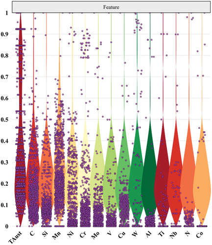
Figure 2. Distribution of M_S in data set.

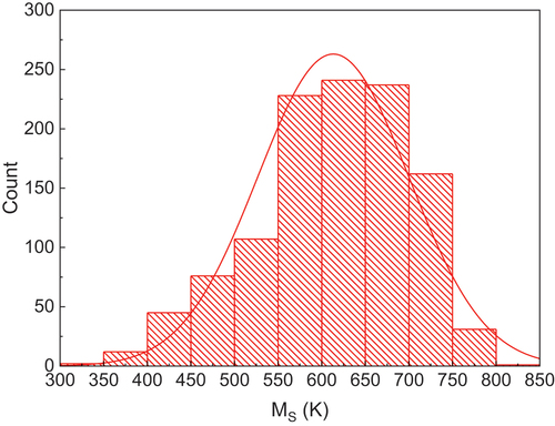
Table 2. Spatial distribution range of data set.

Feature	Description	Max	Min	Mean
TAust	Austenitizing temperature (K)	1673	1023	1256.94
C	wt.% of C	2.25	0.01	0.37
Si	wt.% of Si	3.8	0	0.33
Mn	wt.% of Mn	8	0	0.80
Ni	wt.% of Ni	10	0	0.83
Cr	wt.% of Cr	17	0	1.24
Mo	wt.% of Mo	5.75	0	0.26
V	wt.% of V	5.05	0	0.11
Cu	wt.% of Cu	1.49	0	0.054
W	wt.% of W	19.2	0	0.46
Al	wt.% of Al	1.26	0	0.013
Ti	wt.% of Ti	0.2	0	0.0018
Nb	wt.% of Nb	0.167	0	0.0015
N	wt.% of N	0.287	0	0.0020
Co	wt.% of Co	11.35	0	0.081
MS	Martensite start temperature (K)	819	335	613.26

Table 3. Parameters used in equation (2)(2) $-\mathrm{\Delta }{G}_c(\mathit{J}/\mathit{mol})=K_1+\sqrt{\sum _i{(K_i{X}_i^{0.5})}^2}+\sqrt{\sum _j{(K_j{X}_j^{0.5})}^2}+\sqrt{\sum _k{(K_k{X}_k^{0.5})}^2}+K_{\mathit{Co}}{X}_{Co}^{0.5}$(2) .

Parameter	Value (J/mol)	Parameter	Parameter
KC	4009	KAl	280
KN	3097	KCu	752
KCr	1868	KNi	172
KMn	1980	KW	714
KMo	1418	KCo	352
KNb	1653	KTi	1473
KSi	1979	KV	1618

Table 4. Atomic feature.

Abb.	Description
mAW	mean Atomic Weight
mC	mean Column
mR	mean Row
rN	range Number
mN	mean Number
rAR	range Atomic Radius
mAR	mean Atomic Radius
rE	range Electronegativity
mE	mean Electronegativity
asve	avg s valence electrons
apve	avg p valence electrons
adve	avg d valence electrons
fsve	frac s valence electrons
fpve	frac p valence electrons
fdve	frac d valence electrons
FCC	FCC lattice parameters
BCC	BCC lattice parameters

Table 5. Hyperparametric adjustment.

Model	Hyperparameter	Search range	Optimal hyperparameter
LSO	alpha	[0.1,50]	0.1
ETR	n_estimators	[6], 8000]	1494
	max_depth	[2], 100]	74
	min_samples_split	[2], 100]	2
	min_samples_leaf	[1], 100]	1
	max_features	[0.1,1]	0.82
SVR	C	[1000,8000]	5000
	gamma	[0.1,20]	0.1
GBT	n_estimators	[22], 8000]	3321
	learning_rate	[0.001,1]	0.1
	max_depth	[2,48]	22
	subsample	[0.5,1.0]	0.5
	min_samples_split	[2,48]	19
	min_samples_leaf	[1,16]	1

Figure 3. Comparison of predicted and measured values of four machine learning models with original feature input (a) ETR(b) GBT(c) SVR(d) LOS.

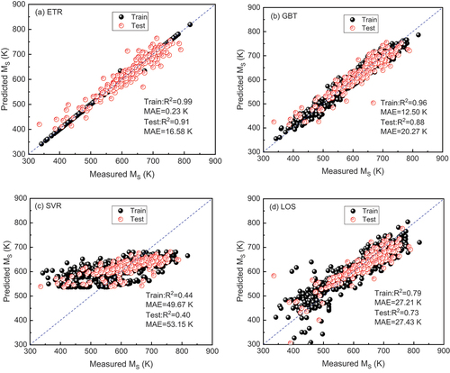
Figure 4. Comparison between the predicted value of the model and the measured value after adding atomic feature.

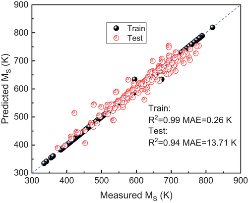
Figure 5. PCC heat map between features.

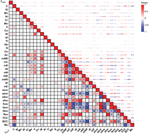
Figure 6. VIF value of multicollinearity feature.

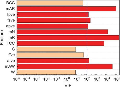
Figure 7. MIC analysis of features and target variables.

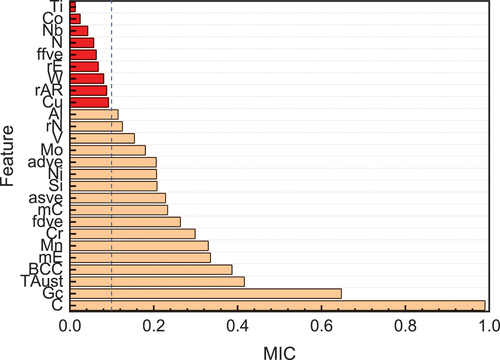
Figure 8. Comparison between predicted values and measured values of the model after feature selection.

Figure 9. Difference between M_S measured value and calculated value.

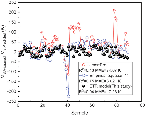
Figure 10. Summary chart of characteristic SHAP values (a) average SHAP(b) SHAP of each sample.

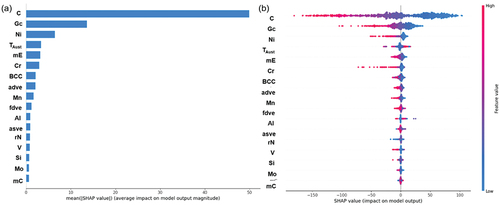
Figure 11. Distribution of SHAP values corresponding to features (a) C (b) gc (c) Ni (d) taust (e) mE (f) Cr (g) BCC (h) adve.

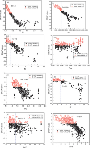
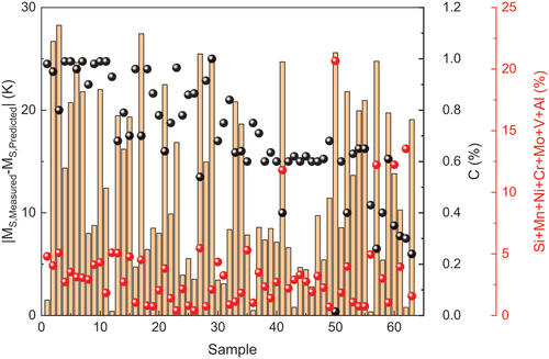
Figure 12. The difference between the calculated value and the measured value of the model and the corresponding C content and element content.

Payson P. Martensite reactions in alloy steels. Trans American Soc Met. 1944;33:261–280.

 Google Scholar

Rowland E. The application of ms points to case depth measurement. Trans ASM. 1946;27(2):27–47. doi: 10.2307/1932518

 Google Scholar

Grange R. The temperature range of martensite formation. Trans American Inst Mining Metal Eng. 1946;167:467–501.

 Google Scholar

Nehrenberg A. The temperature range of martensite formation. Trans AIME. 1946;167:494–498.

 Google Scholar

Steven W. The temperature of martensite and bainite in low-alloy steels. J Iron Steel Inst. 1956;183:349–359.

 Google Scholar

Andrews K. Empirical formulae for the calculation of some transformation temperatures. J Iron Steel Inst. 1965;0:721–727.

 Google Scholar

Kung C, Rayment J. Examination of the validity of existing empirical formulae for the calculation of M/sub s/temperature. Metall Trans A. 1982;13(2):328–331. doi: 10.1007/BF02643327

 Web of Science ®Google Scholar

Ishida K. Calculation of the effect of alloying elements on the ms temperature in steels. Journal of Alloys and Compounds. 1995;220(1–2):126–131. doi: 10.1016/0925-8388(94)06002-9

 Web of Science ®Google Scholar

Sverdlin A, Ness A. Steel heat treatment handbook. GE Totten and MAH Howes, editors. New York: Marcel Dekker Inc.; 1997.

 Google Scholar

Capdevila C, FG C, De Andrés CG. Determination of ms temperature in steels: a bayesian neural network model. ISIJ Inter. 2002;42(8):894–902. doi: 10.2355/isijinternational.42.894

 Web of Science ®Google Scholar

Van Bohemen S. Bainite and martensite start temperature calculated with exponential carbon dependence. Mater Sci Technol. 2012;28(4):487–495. doi: 10.1179/1743284711Y.0000000097

 Web of Science ®Google Scholar

Barbier D. Extension of the martensite transformation temperature relation to larger alloying elements and contents. Adv Eng Mater. 2014;16(1):122–127. doi: 10.1002/adem.201300116

 Web of Science ®Google Scholar

Eichelman G. The effect of composition on. Tran Amer Soc Met. 1953;45:77–95.

 Google Scholar

Finkler H, Schirra M. Transformation behaviour of the high temperature martensitic steels with 8–14% chromium. Steel Res Int. 1996;67(8):328–342. doi: 10.1002/srin.199605498

 Google Scholar

Kaar S, Steineder K, Schneider R, et al. New Ms-formula for exact microstructural prediction of modern 3rd generation AHSS chemistries. Scripta Materialia. 2021;200:113923. doi: 10.1016/j.scriptamat.2021.113923

 Web of Science ®Google Scholar

Lee SJ, Jung M. Prediction of martensite start temperatures of highly alloyed steels. Arch Metallurgy Mat. 2021;66:224. doi: 10.24425/amm.2021.134765

 Web of Science ®Google Scholar

Lee SJ, Park KS. Prediction of martensite start temperature in alloy steels with different grain sizes. Metall Mater Trans A. 2013;44(8):3423–3427. doi: 10.1007/s11661-013-1798-4

 Google Scholar

Liu C, Huang M, Ren Q, et al. Effect of grain size and cooling rate on the martensite start temperature of stainless steel. Steel Res Int. 2022;93(8):2200044. doi: 10.1002/srin.202200044

 Web of Science ®Google Scholar

Yang HS, Bhadeshia H. Uncertainties in dilatometric determination of martensite start temperature. Mater Sci Technol. 2007;23(5):556–14. doi: 10.1179/174328407X176857

 Web of Science ®Google Scholar

Yang HS, Bhadeshia HKDH. Austenite grain size and the martensite-start temperature. Scripta Materialia. 2009;60(7):493–495. doi: 10.1016/j.scriptamat.2008.11.043

 Web of Science ®Google Scholar

L NHK, Nakashima K, Tsuchiyama T, et al. Effect of solution nitriding on microstructure and hardness in 12% Cr martensitic stainless steels. Vol. 98. Kyushu: Tetsu-To-Hagane/Journal of the Iron Steel Institute of Japan; 2012. p. 25–31.

 Google Scholar