Bayesian mean–variance analysis: optimal portfolio selection under parameter uncertainty

Figures & data

Figure 1. The ratio $c_{k,n}/d_n$ plotted as a function of k/n for $k/n\in [0,0.95)$ and $n\in \{50,100\}$.

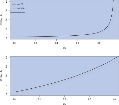
Table 1. Average absolute deviation (AD) of the estimated portfolio expected return and of the estimated portfolio variance from their population values.

$\gamma =50$	AD of portfolio expected return				AD of portfolio variance
Bayesian
Black–Litterman
Sample	n = 50	n = 75	n = 100	n = 130	n = 50	n = 75	n = 100	n = 130
Robust, MVE
Robust, MCD
	0.1017	0.0822	0.0713	0.0621	0.0020	0.0016	0.0014	0.0012
	1.0889	0.7257	0.5438	0.4140	0.0218	0.0145	0.0109	0.0083
k = 5	0.1186	0.0912	0.0768	0.0660	0.0024	0.0018	0.0015	0.0013
	0.3824	0.2284	0.1751	0.1319	0.0076	0.0046	0.0035	0.0026
	0.2494	0.1984	0.1661	0.1459	0.0050	0.0040	0.0033	0.0029
	0.2541	0.1944	0.1660	0.1439	0.0051	0.0039	0.0033	0.0029
	2.6794	1.7051	1.2657	0.9547	0.0536	0.0341	0.0253	0.0191
k = 10	0.4127	0.2730	0.2183	0.1765	0.0083	0.0055	0.0044	0.0035
	1.0597	0.5949	0.4299	0.3305	0.0212	0.0119	0.0086	0.0066
	2.4460	0.9509	0.5799	0.3900	0.0489	0.0190	0.0116	0.0078
	0.8878	0.6205	0.5116	0.4236	0.0178	0.0124	0.0102	0.0085
	8.5916	4.8591	3.3871	2.4422	0.1718	0.0972	0.0677	0.0488
k = 25	3.9959	1.9720	1.3382	0.9466	0.0799	0.0394	0.0268	0.0189
	11.349	5.7082	3.3371	2.1340	0.2269	0.1142	0.0667	0.0427
	25.837	9.3763	5.2220	3.2756	0.5167	0.1875	0.1044	0.0655
	2.3320	1.2120	0.9153	0.7521	0.0466	0.0242	0.0183	0.0150
	16.5132	8.1638	5.1806	3.5884	0.3303	0.1633	0.1036	0.0718
k = 40	27.9857	7.4658	4.2657	2.8229	0.5597	0.1493	0.0853	0.0565
	73.6087	20.148	12.158	7.5067	1.4722	0.4030	0.2432	0.1501
	533.452	33.396	16.574	9.7837	10.669	0.6679	0.3315	0.1957

Notes: The smallest values are depicted in bold. Five considered estimators are the (objective) Bayesian estimator (first line in each panel), the estimator resulting from the (extended) Black–Litterman model (second line in each panel), the sample estimator (third line in each panel), the robust MVE estimator (fourth line in each panel), and the robust MCD estimator (fifth line in each panel) for several values of $k\in \{5,10,25,40\}$ and $n\in \{50,75,100,130\}$ with $\gamma =50$. The asset returns are assumed to be conditionally normally distributed with small variances.

Table 2. Average absolute deviation (AD) of the estimated portfolio expected return and of the estimated portfolio variance from their population values.

$\gamma =50$	AD of portfolio expected return				AD of portfolio variance
Bayesian
Black–Litterman
Sample	n = 50	n = 75	n = 100	n = 130	n = 50	n = 75	n = 100	n = 130
Robust, MVE
Robust, MCD
	0.0111	0.0091	0.0079	0.0070	0.0002	0.0002	0.0002	0.0001
	0.0932	0.0629	0.0473	0.0361	0.0018	0.0012	0.0009	0.0007
k = 5	0.0133	0.0102	0.0086	0.0075	0.0003	0.0002	0.0002	0.0001
	0.0292	0.0192	0.0154	0.0123	0.0006	0.0004	0.0003	0.0002
	0.0389	0.0234	0.0177	0.0132	0.0008	0.0005	0.0003	0.0003
	0.0256	0.0200	0.0171	0.0147	0.0005	0.0004	0.0003	0.0003
	0.2397	0.1542	0.1155	0.0874	0.0048	0.0031	0.0023	0.0017
k = 10	0.0431	0.0287	0.0229	0.0184	0.0009	0.0006	0.0005	0.0004
	0.1079	0.0600	0.0435	0.0331	0.0021	0.0012	0.0009	0.0007
	0.2498	0.0956	0.0584	0.0390	0.0050	0.0019	0.0012	0.0008
	0.0878	0.0619	0.0512	0.0428	0.0018	0.0012	0.0010	0.0009
	0.7786	0.4504	0.3171	0.2310	0.0156	0.0090	0.0063	0.0046
k = 25	0.4062	0.2003	0.1355	0.0966	0.0081	0.0040	0.0027	0.0019
	1.1483	0.5773	0.3361	0.2148	0.0230	0.0115	0.0067	0.0043
	2.6215	0.9502	0.5253	0.3290	0.0524	0.0190	0.0105	0.0066
	0.2280	0.1200	0.0915	0.0747	0.0046	0.0024	0.0018	0.0015
	1.4380	0.7473	0.4825	0.3379	0.0288	0.0149	0.0096	0.0068
k = 40	2.8277	0.7556	0.4309	0.2848	0.0565	0.0151	0.0086	0.0057
	7.3905	2.0316	1.2234	0.7575	0.1478	0.0406	0.0245	0.0151
	52.933	3.3593	1.6674	0.9872	1.0587	0.0672	0.0333	0.0197

Notes: The smallest values are depicted in bold. The five estimators are the (objective) Bayesian estimator (first line in each panel), the estimator resulting from the (extended) Black–Litterman model (second line in each panel), the sample estimator (third line in each panel), the robust MVE estimator (fourth line in each panel), and the robust MCD estimator (fifth line in each panel) for several values of $k\in \{5,10,25,40\}$ and $n\in \{50,75,100,130\}$ with $\gamma =50$. The asset returns are assumed to be conditionally normally distributed with large variances.

Table 3. Average absolute deviation (AD) of the estimated portfolio expected return and of the estimated portfolio variance from their population values.

$\gamma =50$	AD of portfolio expected return				AD of portfolio variance
Bayesian
Black–Litterman
Sample	n = 50	n = 75	n = 100	n = 130	n = 50	n = 75	n = 100	n = 130
Robust, MVE
Robust, MCD
	0.1490	0.1209	0.1088	0.0956	0.0030	0.0024	0.0022	0.0019
	1.2668	0.8216	0.6116	0.4632	0.0253	0.0164	0.0122	0.0093
k = 5	0.1971	0.1480	0.1268	0.1076	0.0039	0.0030	0.0025	0.0022
	0.7206	0.5815	0.5211	0.4857	0.0144	0.0116	0.0104	0.0097
	0.7974	0.6005	0.5240	0.4836	0.0159	0.0120	0.0105	0.0097
	0.3728	0.3008	0.2633	0.2272	0.0075	0.0060	0.0053	0.0045
	3.3112	2.0669	1.5232	1.1441	0.0662	0.0413	0.0305	0.0229
k = 10	0.7125	0.4794	0.3833	0.3089	0.0143	0.0096	0.0077	0.0062
	2.3178	1.6962	1.4892	1.3501	0.0464	0.0339	0.0298	0.0270
	3.6668	2.1039	1.6832	1.4458	0.0733	0.0421	0.0337	0.0289
	1.4528	1.1011	0.9058	0.7880	0.0291	0.0220	0.0181	0.0158
	11.873	6.8656	4.7531	3.4785	0.2374	0.1373	0.0951	0.0696
k = 25	6.8816	3.5138	2.3958	1.7749	0.1376	0.0703	0.0479	0.0355
	18.522	10.176	7.0974	5.6988	0.3704	0.2035	0.1419	0.1140
	29.560	14.142	10.194	8.1919	0.5912	0.2828	0.2039	0.1638
	3.2387	2.3571	1.9424	1.6140	0.0648	0.0471	0.0388	0.0323
	22.5595	12.4591	8.3420	5.9158	0.4512	0.2492	0.1668	0.1183
k = 40	46.3159	12.7395	7.5904	5.1566	0.9263	0.2548	0.1518	0.1031
	117.427	33.2640	20.775	14.454	2.3485	0.6653	0.4155	0.2891
	541.115	42.8432	25.721	18.805	10.822	0.8569	0.5144	0.3761

Notes: The smallest values are depicted in bold. The five estimators are the (objective) Bayesian estimator (first line in each panel), the estimator resulting from the (extended) Black–Litterman model (second line in each panel), the sample estimator (third line in each panel), the robust MVE estimator (fourth line in each panel), and the robust MCD estimator (fifth line in each panel) for several values of $k\in \{5,10,25,40\}$ and $n\in \{50,75,100,130\}$ with $\gamma =50$. The asset returns are assumed to be conditionally multivariate t-distributed with 5 degrees of freedom and small variances.

Table 4. Average absolute deviation (AD) of the estimated portfolio expected return and of the estimated portfolio variance from their population values.

$\gamma =50$	AD of portfolio expected return				AD of portfolio variance
Bayesian
Black–Litterman
Sample	n = 50	n = 75	n = 100	n = 130	n = 50	n = 75	n = 100	n = 130
Robust, MVE
Robust, MCD
	0.0150	0.0123	0.0110	0.0096	0.0003	0.0002	0.0002	0.0002
	0.1085	0.0710	0.0533	0.0405	0.0021	0.0014	0.0010	0.0008
k = 5	0.0196	0.0149	0.0127	0.0107	0.0004	0.0003	0.0003	0.0002
	0.0671	0.0528	0.0472	0.0436	0.0013	0.0010	0.0009	0.0009
	0.0737	0.0544	0.0475	0.0435	0.0014	0.0011	0.0009	0.0008
	0.0374	0.0300	0.0263	0.0225	0.0007	0.0006	0.0005	0.0004
	0.2958	0.1863	0.1386	0.1043	0.0059	0.0037	0.0028	0.0021
k = 10	0.0706	0.0474	0.0379	0.0303	0.0014	0.0009	0.0008	0.0006
	0.2242	0.1613	0.1412	0.1271	0.0045	0.0032	0.0028	0.0025
	0.3534	0.1998	0.1592	0.1361	0.0070	0.0040	0.0032	0.0027
	0.1476	0.1116	0.0912	0.0792	0.0023	0.0022	0.0018	0.0015
	1.0651	0.6335	0.4441	0.3277	0.0213	0.0127	0.0089	0.0065
k = 25	0.6878	0.3502	0.2383	0.1763	0.0137	0.0070	0.0048	0.0035
	1.8374	1.0074	0.6999	0.5614	0.0367	0.0201	0.0140	0.0112
	2.9172	1.3960	1.0026	0.8062	0.0583	0.0279	0.0200	0.0161
	0.3257	0.2392	0.1970	0.1630	0.0065	0.0048	0.0039	0.0033
	1.9528	1.1312	0.7753	0.5575	0.0391	0.0226	0.0155	0.0111
k = 40	4.6225	1.2720	0.7580	0.5142	0.0924	0.0254	0.0152	0.0103
	11.768	3.3082	2.0689	1.4391	0.2354	0.0662	0.0414	0.0288
	49.947	4.2723	2.5567	1.8670	0.9989	0.0854	0.0511	0.0373

Notes: The smallest values are depicted in bold. The five estimators are the (objective) Bayesian estimator (first line in each panel), the estimator resulting from the (extended) Black–Litterman model (second line in each panel), the sample estimator (third line in each panel), the robust MVE estimator (fourth line in each panel), and the robust MCD estimator (fifth line in each panel) for several values of $k\in \{5,10,25,40\}$ and $n\in \{50,75,100,130\}$ with $\gamma =50$. The asset returns are assumed to be conditionally multivariate t-distributed with 5 degrees of freedom and large variances.

Figure 2. Sample optimal portfolios (squares), (objective) Bayesian optimal portfolios (circles), and the Black–Litterman optimal portfolios (triangulares) for the risk aversion coefficient of $\gamma \in \{10,25,50,100\}$, for the sample case of n = 130 and for the portfolio dimension of $k\in \{5,10,25,40\}$ in the case of weekly data.

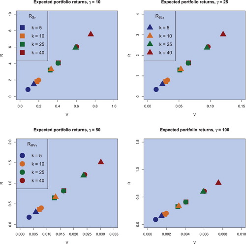
Figure 3. The sample efficient frontier, the (objective) Bayesian efficient frontier, and the Black–Litterman efficient frontier for n = 130 and $k\in \{5,10,25,40\}$ in the case of weekly data.

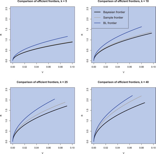
Figure 4. The sample efficient frontier, the (objective) Bayesian efficient frontier, and the Black–Litterman efficient frontier for k = 40 and $n\in \{52,78,104,130\}$ in the case of weekly data.

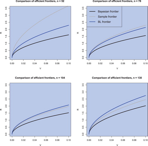
Figure 5. Sample optimal portfolios (squares), (objective) Bayesian optimal portfolios (circles), and the Black–Litterman optimal portfolios (triangulares) for the risk aversion coefficient of $\gamma \in \{10,25,50,100\}$, for the sample case of n = 130 and for the portfolio dimension of $k\in \{5,10,25,40\}$ in the case of monthly data.

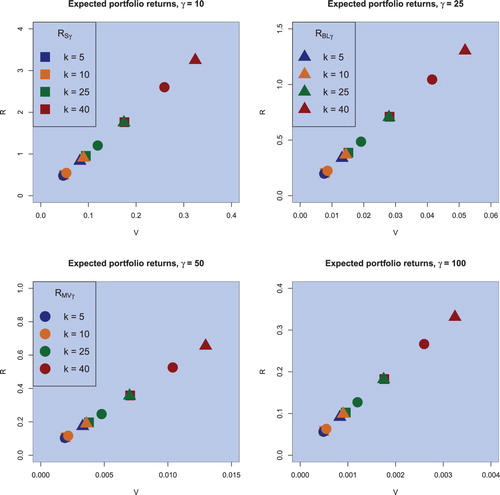
Figure 6. The sample efficient frontier, the (objective) Bayesian efficient frontier, and the Black–Litterman efficient frontier for n = 130 and $k\in \{5,10,25,40\}$ in the case of monthly data.

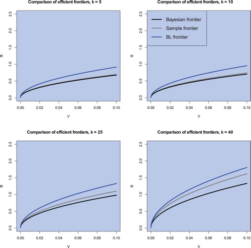
Figure 7. The sample efficient frontier, the (objective) Bayesian efficient frontier, and the Black–Litterman efficient frontier for k = 40 and $n\in \{52,78,104,130\}$ in the case of monthly data.

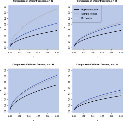
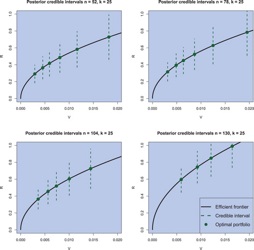
Figure 8. Credible intervals for the return of optimal portfolios with varying risk attitudes for weekly data obtained by employing the (objective) Bayesian approach. The sample sizes are chosen to be $n\in \{52,78,104,130\}$ and the portfolio dimension is fixed to k = 25. The confidence level is set to $\alpha =0.05$.

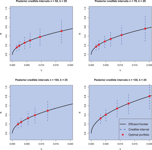
Figure 9. Credible intervals for the return of optimal portfolios for the Black–Litterman model with varying risk attitudes for weekly data. The sample sizes are chosen to be $n\in \{52,78,104,130\}$ and the portfolio dimension is fixed to k = 25. The confidence level is set to $\alpha =0.05$.

Figure 10. Credible intervals for the return of optimal portfolios with varying risk attitudes for monthly data obtained by employing the (objective) Bayesian approach. The sample sizes are chosen to be $n\in \{52,78,104,130\}$ and the portfolio dimension is fixed to k = 25. The confidence level is set to $\alpha =0.05$.

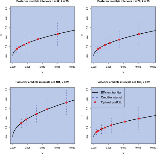
Figure 11. Credible intervals for the return of optimal portfolios for the Black–Litterman model with varying risk attitudes for monthly data. The sample sizes are chosen to be $n\in \{52,78,104,130\}$ and the portfolio dimension is fixed to k = 25. The confidence level is set to $\alpha =0.05$.