Optimal portfolio allocation and asset centrality revisited

Figures & data

Figure 1. FTSE 100 Index. Centrality measures and portfolio weights. Panel (a) reports the relationship between asset centrality and the portfolio weights. To do this, the weights allocated to the assets comprising the FTSE 100 Index under the global minimum variance portfolio, see (2(2) ${\mathbf{w}}^{\ast }=\frac{{\mathbf{\Sigma }}^{-1}\mathbf{1}}{{\mathbf{1}}^{\mathrm{\prime }}{\mathbf{\Sigma }}^{-1}\mathbf{1}}.$(2) ), are ranked from smallest to largest and the associated centrality measure (9(9) $v_i={\overline{\omega }}^{-1}\sum _{j=1}^n{\mathrm{\Omega }}_{ij}{v}_j,$(9) ) is plotted. Panel (b) reports the relationship between asset centrality and the portfolio weights under short-selling constraints $\mathbf{w}\ge 0$.

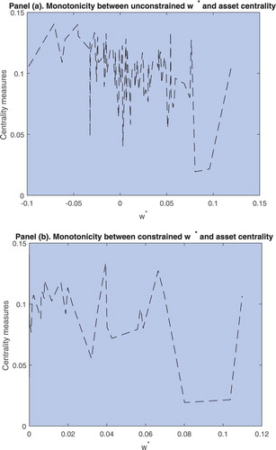
Figure 2. Random subsample of FTSE 100 Index. Centrality measures and portfolio weights. Each row contains a random subsample of 20 stock returns from the FTSE 100 Index such that the five rows span all the assets in the FTSE 100 Index. The left panel reports the relationship between asset centrality and the portfolio weights under the absence of short-selling constraints and the right panel reports such relationship imposing short-selling constraints ($\mathbf{w}\ge 0$).

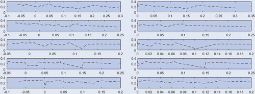
Table 1. Summary statistics. January 2011 to May 2020.

Variable	Obs	Mean	Std. Dev.	Min	Max
Gold ETF Vol	2,362	−0.002	5.544	−30.692	48.07
U.S./Euro	2,362	−0.007	0.761	−18.609	18.77
DJIA	2,362	0.033	1.098	−13.841	10.76
Nasdaq	2,362	0.061	1.234	−13.001	9.596
Russell 2000 Vol	2,362	0.019	6.254	−36.428	54.04
S$\mathrm{\&}$P 500	2,362	0.037	1.098	−12.765	8.968
VIX	2,362	0.018	7.977	−31.414	76.82
Willshire 5000	2,362	0.035	1.115	−13.110	8.984

Figure 3. Static analysis of centrality measures and portfolio weights. Panels (a)–(f): the black solid line denotes the positive centrality measure (10(10) $v_i^p={\overline{\lambda }}_1^{-1}\sum _{j=1}^n{\mathrm{\Lambda }}_{1,ij}{v}_j^p,$(10) ) and the red dashed line the negative measure (11(11) $v_i^n={\overline{\lambda }}_2^{-1}\sum _{j=1}^n{\mathrm{\Lambda }}_{2,ij}{v}_j^n,$(11) ). Panel (a): the green line denotes the centrality measure (9(9) $v_i={\overline{\omega }}^{-1}\sum _{j=1}^n{\mathrm{\Omega }}_{ij}{v}_j,$(9) ). Panel (b): the red line for the constrained portfolio and blue dashed line for the unconstrained portfolio. Panels (c)–(d): the blue dashed line denotes the optimal portfolio allocation for each asset. Panels (e)–(f): the blue dashed line denotes the centrality measure (9(9) $v_i={\overline{\omega }}^{-1}\sum _{j=1}^n{\mathrm{\Omega }}_{ij}{v}_j,$(9) ).

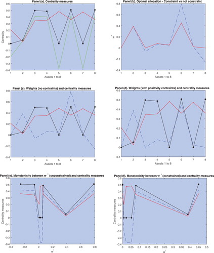
Figure 4. CCC model with constrained weights. The black solid line denotes the positive centrality measure (10(10) $v_i^p={\overline{\lambda }}_1^{-1}\sum _{j=1}^n{\mathrm{\Lambda }}_{1,ij}{v}_j^p,$(10) ) and the red dashed line the negative centrality measure (11(11) $v_i^n={\overline{\lambda }}_2^{-1}\sum _{j=1}^n{\mathrm{\Lambda }}_{2,ij}{v}_j^n,$(11) ). The blue line denotes the dynamic optimal portfolio allocation over the evaluation period January 2011 to May 2020.

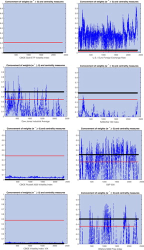
Figure 5. DCC model with constrained weights. The black solid line denotes the positive centrality measure (10(10) $v_i^p={\overline{\lambda }}_1^{-1}\sum _{j=1}^n{\mathrm{\Lambda }}_{1,ij}{v}_j^p,$(10) ) and the red dashed line the negative centrality measure (11(11) $v_i^n={\overline{\lambda }}_2^{-1}\sum _{j=1}^n{\mathrm{\Lambda }}_{2,ij}{v}_j^n,$(11) ). The blue line denotes the dynamic optimal portfolio allocation over the evaluation period January 2011 to May 2020.

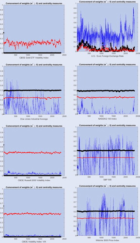
Table 2. Covariance and correlation matrix. January 2011 to May 2020.

Sample covariance matrix
Variable	Gold ETF Vol	U.S./Euro	DJIA	Nasdaq	Russell 2000 Vol	S$\mathrm{\&}$P 500	VIX	Willshire 5000
Gold ETF Vol	30.737
U.S./Euro	−0.207	0.579
DJIA	−1.924	0.064	1.207
Nasdaq	−2.081	0.056	1.202	1.524
Russell 2000 Vol	14.694	−0.255	−4.953	−5.754	39.122
S$\mathrm{\&}$P 500	−2.016	0.069	1.179	1.271	−5.214	1.206
VIX	18.357	−0.284	−6.242	−7.265	45.052	−6.573	63.637
Willshire 5000	−2.055	0.071	1.191	1.286	−5.334	1.222	−6.658	1.243
Sample correlation matrix
Variable	Gold ETF Vol	U.S./Euro	DJIA	Nasdaq	Russell 2000 Vol	S$\mathrm{\&}$P 500	VIX	Willshire 5000
Gold ETF Vol	1
U.S./Euro	−0.049	1
DJIA	−0.316	0.077	1
Nasdaq	−0.304	0.059	0.886	1
Russell 2000 Vol	0.424	−0.053	−0.721	−0.745	1
S$\mathrm{\&}$P 500	−0.331	0.083	0.977	0.937	−0.759	1
VIX	0.415	−0.046	−0.712	−0.737	0.903	−0.750	1
Willshire 5000	−0.332	0.084	0.972	0.934	−0.765	0.998	−0.748	1

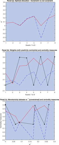
Figure 6. Static analysis of centrality measures and portfolio weights. Panel (a): the red line denotes the constrained portfolio and the blue dashed line the unconstrained portfolio. Panel (b): the black solid line denotes the positive centrality measure (10(10) $v_i^p={\overline{\lambda }}_1^{-1}\sum _{j=1}^n{\mathrm{\Lambda }}_{1,ij}{v}_j^p,$(10) ) and the red dashed line the negative centrality measure (11(11) $v_i^n={\overline{\lambda }}_2^{-1}\sum _{j=1}^n{\mathrm{\Lambda }}_{2,ij}{v}_j^n,$(11) ). The blue dashed line denotes the optimal portfolio allocation for each asset. Panel (c): the black solid line denotes the positive centrality measure (10(10) $v_i^p={\overline{\lambda }}_1^{-1}\sum _{j=1}^n{\mathrm{\Lambda }}_{1,ij}{v}_j^p,$(10) ) and the red dashed line the negative centrality measure (11(11) $v_i^n={\overline{\lambda }}_2^{-1}\sum _{j=1}^n{\mathrm{\Lambda }}_{2,ij}{v}_j^n,$(11) ). The blue dashed line denotes the centrality measure (9(9) $v_i={\overline{\omega }}^{-1}\sum _{j=1}^n{\mathrm{\Omega }}_{ij}{v}_j,$(9) ).

Table 3. CCC and DCC correlation matrices. January 2011 to May 2020.

CCC correlation matrix
Variable	Gold ETF Vol	U.S./Euro	DJIA	Nasdaq	Russell 2000 Vol	S$\mathrm{\&}$P 500	VIX	Willshire 5000
Gold ETF Vol	1
U.S./Euro	−0.056	1
DJIA	−0.346	0.080	1
Nasdaq	−0.321	0.056	0.847	1
Russell 2000 Vol	0.432	−0.046	−0.766	−0.757	1
S$\mathrm{\&}$P 500	−0.362	0.080	0.963	0.922	−0.809	1
VIX	0.425	−0.047	−0.801	−0.778	0.899	−0.838	1
Willshire 5000	−0.363	0.079	0.956	0.920	−0.820	0.997	−0.837	1
DCC correlation matrix
Variable	Gold ETF Vol	U.S./Euro	DJIA	Nasdaq	Russell 2000 Vol	S$\mathrm{\&}$P 500	VIX	Willshire 5000
Gold ETF Vol	1
U.S./Euro	−0.062	1
DJIA	−0.317	0.107	1
Nasdaq	−0.286	0.079	0.847	1
Russell 2000 Vol	0.412	−0.074	−0.766	−0.750	1
S$\mathrm{\&}$P 500	−0.331	0.109	0.964	0.920	−0.808	1
VIX	0.402	−0.073	−0.796	−0.764	0.902	−0.830	1
Willshire 5000	−0.332	0.107	0.957	0.918	−0.818	0.997	−0.830	1
${\lambda }_1$	0.020${}^{\ast \ast \ast }$
${\lambda }_2$	0.945${}^{\ast \ast \ast }$