Optimal trade execution for Gaussian signals with power-law resilience

Figures & data

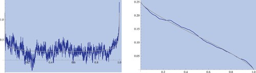
Figure 1. On the left we have plotted the optimal inventory $X_t^{\ast }$ in Theorem 2.2 when $P_t=\sigma {\int }_0^t(t-s{)}^{H-\frac{1}{2}}\mathrm{d}{W}_s$ is a Riemann-Liouville process using (26(26) $\begin{array}{rl}k(u,t)& =-\left(2c{\pi }^{\frac{3}{2}}{\tau }^{\frac{3}{2}}{\overline{u}}^{\frac{1}{4}}\mathrm{\Gamma }\right(H){)}^{-1}\cdot \left[\frac{{\tau }^{\frac{3}{2}+H}\sigma \mathrm{\Gamma }\left(\frac{1}{4}\right)\mathrm{\Gamma }\left(H_{\frac{1}{4}}\right)}{w^{\frac{1}{4}}(u-t)}\right.\\ & +H_{\frac{1}{4}}{\tau }^{\frac{1}{2}+H}{\overline{u}}^{-\frac{3}{4}+H}\sigma \mathrm{\Gamma }\left(\frac{1}{4}\right)\left(-B\left(\overline{u},-H_{\frac{1}{4}},\frac{3}{4}\right)\right.\\ & +\left.\frac{\mathrm{\Gamma }\left(\frac{3}{4}\right)\mathrm{\Gamma }\left(-H_{\frac{1}{4}}\right)}{\mathrm{\Gamma }(\frac{1}{2}-H)}\right)\mathrm{\Gamma }\left(H_{\frac{1}{4}}\right)\\ & \left.+\frac{\sqrt{2\pi }\mathrm{\Gamma }\left(H\right)({\tau }^{\frac{1}{2}+H}\sigma +\tau {\lambda }_1(u\left)\right)}{w^{\frac{1}{4}}}\right],\end{array}$(26) ) with $H=\frac{2}{3}$, $\sigma =1$, c = 1 and $\gamma =.5$ and $X_0=0$, and in the middle we have plotted $u_t^{\ast }$ (blue) and ${\xi }_t$ (in red). On the right, as a sanity check, we have plotted the expected profit/loss for α times the optimal trading speed, as a function of α (which we see is correctly maximized close to $\alpha =1$, the small numerical error is there because we have to estimate the triple integral in (24) with Monte Carlo).

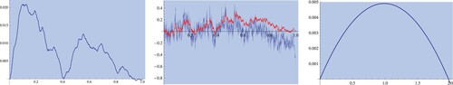
Figure 2. Non-Round trip case: from left to right (with $X_0=.25$ and the same parameters as above) we see (i) the optimal buying speed with no-signal (ii) $X_t^{\ast }$ with no signal.

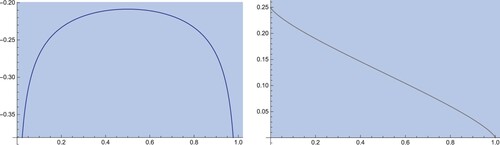
Figure 3. On the left we see the optimal selling speed with non-zero signal (blue) and the no-signal optimal speed (grey) and on the right we see $X_t^{\ast }$ with non-zero signal (blue) and zero signal (grey), for the same parameters and simulated Brownian motion as figure 2.