State-dependent Hawkes processes and their application to limit order book modelling

Figures & data

Figure 1. Simulation of a state-dependent Hawkes process with $d_e=1$, $d_x=2$. The upper plot shows the evolution of the state process. The blue dots indicate the event times and the lower plot represents the intensity. The process is specified so that ${\nu }_1=1$ and $k_{11}(t,x)=\exp (-4t){\text{1}}_{\{x=2\}}$, that is, in state 2 the process exhibits exponential self-excitation whereas no self-excitation occurs in state 1.

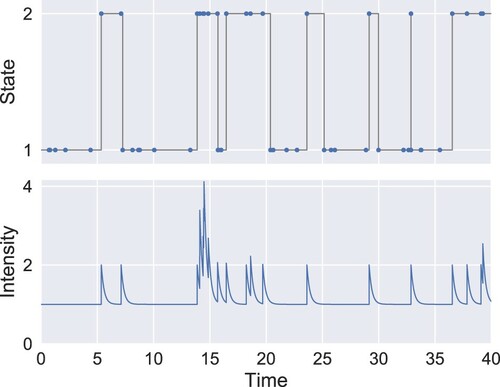
Figure 2. Descriptive statistics of level-I order flow of INTC. Except for Figure 2(a), only the data between 12:00 and 14:30 are used. In Figure 2(a), the sample mean of the arrival rate of level-I orders is computed over 10-minute bins. The translucent area represents the range of the arrival rate across the 250 trading days, excluding the bottom and top 5% values. (a) Arrival rate of level-I orders. (b) Number of level-I orders. (c) Fraction of level-I orders with non-unique timestamp. (d) Distribution of level-I order types.

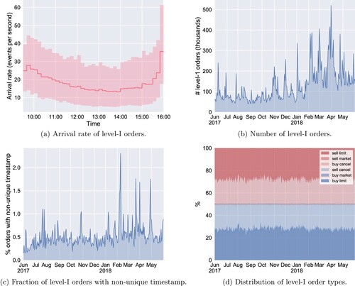
Figure 3. Joint distribution of events and states for INTC, depicting the empirical distribution of the marks $(E_n,X_n)$ for the two considered state processes. (a) ${\text{Model}}_{\text{S}}$ (state process: bid–ask spread). (b) ${\text{Model}}_{\text{QI}}$ (state process: queue imbalance).

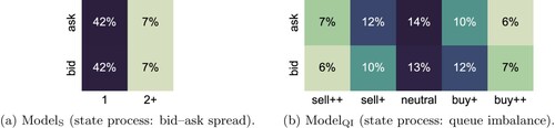
Table 1. Summary of ${\text{Model}}_{\text{S}}$ and ${\text{Model}}_{\text{QI}}$.

	${\text{Model}}_{\text{S}}$	${\text{Model}}_{\text{QI}}$
Event types	ask and bid events, $d_e=2$, $\mathcal{E}=\left\{ask,bid\right\}$
State process	Bid–ask spread, $d_x=2$  $\mathcal{X}=\{1,\mathbf{\text{{ 2+}}}\}$	Queue imbalance, $d_x=5$  $\mathcal{X}=\{\mathbf{\text{{ sell++}}},\mathbf{\text{{ sell+}}},\mathbf{\text{{ neutral}}},\mathbf{\text{{ buy+}}},\mathbf{\text{{ buy++}}}\}$
Kernel $\mathit{k}$	Exponential, of the form (6(6) $k_{e^{\prime }e}(t,x)={\alpha }_{e^{\prime }xe}\exp (-{\text{β}}_{e^{\prime }xe}t),t>0,e^{\prime },e\in \mathcal{E},x\in \mathcal{X},$(6) )
No. of parameters	26	92

Figure 4. Estimated transition distributions $\hat{\mathit{\varphi }}$ of ${\text{Model}}_{\text{S}}$ and ${\text{Model}}_{\text{QI}}$. We report the average of ${\hat{\mathit{\varphi }}}^{\left(i\right)}$ across the 250 trading days. (Daily estimates vary little from these averaged values.). (a) Transition probabilities of the bid–ask spread (${\text{Model}}_{\text{S}}$). (b) Transition probabilities of the queue imbalance (${\text{Model}}_{\text{QI}}$).

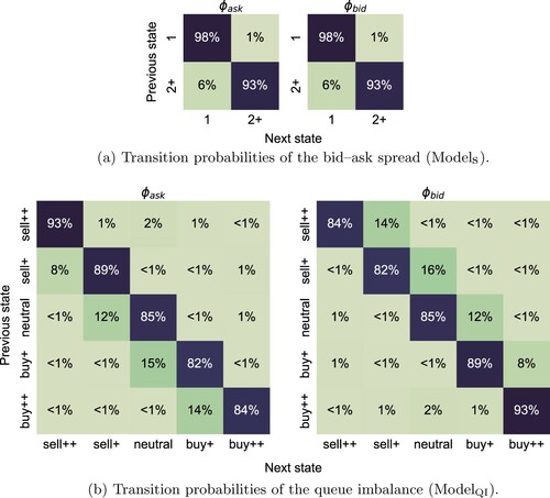
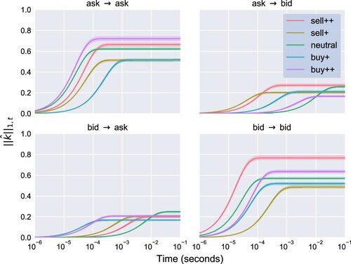
Figure 5. The estimated kernel $\hat{\mathit{k}}$ under ${\text{Model}}_{\text{S}}$ and ${\text{Model}}_{\text{QI}}$. Each panel describes self- or cross-excitation as indicated by its title, whilst each colour corresponds to a different state. For example, in Figure 5(a), the red curves in the second panel represent the estimates ${\hat{k}}_{e^{\prime }e}^{\left(i\right)}(\cdot ,x)$ where $e^{\prime }=\mathbf{\text{{ ask}}}$, $e=\mathbf{\text{{ bid}}}$ and $x=\mathbf{\text{{ 1}}}$. All daily estimates are superposed with one translucent curve for each day. An ‘aggregate’ kernel is represented by a solid line, computed using the median of ${\hat{\mathit{\alpha }}}^{\left(i\right)}$ and ${\widehat{\text{β}}}^{\left(i\right)}$ across the 250 trading days. (a) ${\text{Model}}_{\text{S}}$ (state variable: bid–ask spread). (b) ${\text{Model}}_{\text{QI}}$ (state variable: queue imbalance).

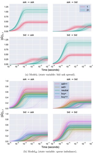
Figure 6. Estimated base rate vector ${\hat{\mathit{\nu }}}^{\left(i\right)}$ for ${\text{Model}}_{\text{S}}$ and ${\text{Model}}_{\text{QI}}$ over time (in number of events per second). (a) ${\text{Model}}_{\text{S}}$. (b) ${\text{Model}}_{\text{QI}}$.

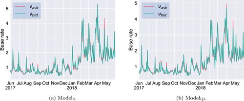
Figure 7. Estimated kernel norms $\Vert \hat{\mathit{k}}{\Vert }_{1,\mathrm{\infty }}$ for ${\text{Model}}_{\text{QI}}$ over time. The dashed line marks 5 February 2018 (‘the return of volatility’), a day when the CBOE Volatility Index (VIX) jumped by 116% to 38 points, a level not seen since August 2015. This day seems to have introduced a systematic change in the magnitude of cross- and self-excitation. The spike in cross-excitation that occurs on 21 February 2018 is linked to a sudden change in market behaviour around 14:00 on that day, when Intel Corporation rolled out patches for its most recent generation of processors.

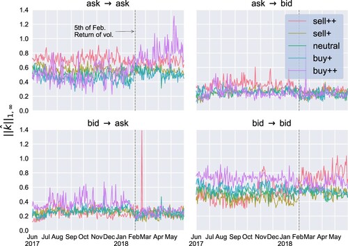
Figure 8. The upper panel depicts the evolution of the queue imbalance and level-I order flow of INTC on 13 February 2018 and the ask (red dots) and bid (blue dots) events. The lower panel displays the estimated intensities of ${\text{Model}}_{\text{QI}}$. (The self- and cross-excitation kernel norms of ${\text{Model}}_{\text{QI}}$ on 13 February 2018 are visualised in Figure A2.)

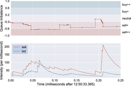
Figure 9. In-sample (12:00–14:30) and out-of-sample (14:30–15:00) Q–Q plots of event residuals under ${\text{Model}}_{\text{S}}$, ${\text{Model}}_{\text{QI}}$ (state-dependent) and an ordinary Hawkes process (simple). The residuals of the ith day are computed using the ML estimates $({\hat{\mathit{\nu }}}^{\left(i\right)},{\hat{\mathit{\alpha }}}^{\left(i\right)},{\widehat{\text{β}}}^{\left(i\right)})$ obtained from the 12:00–14:30 period. The empirical quantiles are obtained by pooling the residuals of all 250 trading days. The two panels in each sub-figure correspond to the sequences of residuals $\left(r_n^e\right)$ for $e\in \mathcal{E}=\{\mathrm{a}\mathrm{s}\mathrm{k},\mathrm{b}\mathrm{i}\mathrm{d}\}$. (a) ${\text{Model}}_{\text{S}}$: in sample. (b) ${\text{Model}}_{\text{S}}$: out of sample. (c) ${\text{Model}}_{\text{QI}}$: in sample. (d) ${\text{Model}}_{\text{QI}}$: out of sample.

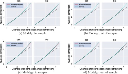
Figure 10. The estimated spectral radius $\hat{\rho }\left(x\right)$ as a function of $x\in \mathcal{X}$ under ${\text{Model}}_{\text{S}}$ and ${\text{Model}}_{\text{QI}}$. The daily profiles $x\mapsto \hat{\rho }(x{)}^{\left(i\right)}$, $i=1,\dots ,250$, are represented by the red translucent curves. (a) ${\text{Model}}_{\text{S}}$. (b) ${\text{Model}}_{\text{QI}}$.

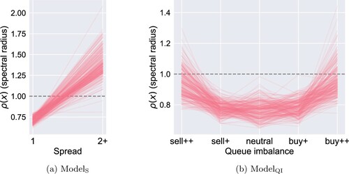
Figure 11. In-sample (12:00–14:30) Q–Q plots of total residuals of ${\text{Model}}_{\text{QI}}$ (state-dependent) and the alternative model given by (8(8) $\begin{array}{rl}{\tilde{\lambda }}_{ex}\left(t\right)& ={\nu }_{ex}+\sum _{e^{\prime }\in \mathcal{E},x^{\prime }\in \mathcal{X}}{\int }_{[0,t)}{k}_{e^{\prime }{x}^{\prime }ex}(t-s)\mathrm{d}{\tilde{N}}_{e^{\prime }{x}^{\prime }}\left(s\right),t\ge 0,\\ & e\in \mathcal{E},x\in \mathcal{X},\end{array}$(8) ) (complex) on 11 May 2018. Each panel corresponds to a sequence of residuals $\left({\tilde{r}}_n^{ex}\right)$ for all $e\in \mathcal{E}$ and $x\in \mathcal{X}$.

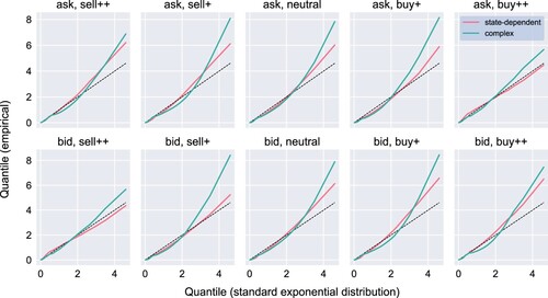
Table A1. Parameter values for Specification 1.

(a) Impact coefficients.
${\alpha }_{i1j}$		${\alpha }_{i2j}$		${\alpha }_{i3j}$		${\alpha }_{i4j}$		${\alpha }_{i5j}$
11,314	2,311	8,098	3,556	17,016	270	3,198	535	34,747	220
139	33,460	724	4,497	178	15,497	3,778	7,943	2,353	12,452
(b) Decay coefficients.
${\text{β}}_{i1j}$		${\text{β}}_{i2j}$		${\text{β}}_{i3j}$		${\text{β}}_{i4j}$		${\text{β}}_{i5j}$
17,480	9,563	15,187	19,637	29,890	1,456	6,493	3,071	45,546	1,097
613	44,994	4,614	8,384	1,026	27,522	20,537	14,272	10,443	18,988
(c) Transition distribution.
${\varphi }_1(i,j)$					${\varphi }_2(i,j)$
.89	.02	.05	.03	.01	.78	.19	.02	<.01	<.01
.13	.83	.01	<.01	.02	<.01	.75	.2	.02	<.01
.02	.17	.79	<.01	.02	.02	<.01	.79	.17	.02
<.01	.02	.21	.75	.01	.02	<.01	<.01	.82	.14
<.01	<.01	.02	.19	.78	<.01	.03	.06	.02	.89
(d) Base rate vector.
${\nu }_i$
2.2
2.2

Table A2. Parameter values for Specification 2.

(a) Impact coefficients.
${\alpha }_{i1j}$		${\alpha }_{i2j}$		${\alpha }_{i3j}$		${\alpha }_{i4j}$		${\alpha }_{i5j}$
2	10	1	3	1,000	30	2,000	40	100	1,000
10	2	3	1	20	3,000	2,000	50	60	2,000
(b) Decay coefficients.
${\text{β}}_{i1j}$		${\text{β}}_{i2j}$		${\text{β}}_{i3j}$		${\text{β}}_{i4j}$		${\text{β}}_{i5j}$
10	15	8	4	3,000	500	6,000	160	500	8,000
15	10	4	8	1000	5,000	10,000	300	120	5,000
(c) Transition distribution.
${\varphi }_1(i,j)$					${\varphi }_2(i,j)$
.7	.3	.0	.0	.0	.0	.1	.2	.3	.4
.1	.8	.1	.0	.0	.2	.1	.4	.2	.1
.0	.1	.6	.2	.1	.1	.3	.1	.3	.2
.2	.2	.3	.1	.2	.0	.0	.1	.8	.1
.1	.3	.3	.1	.2	.1	.0	.1	.1	.7
(d) Base rate vector.
${\nu }_i$
5
1

Figure A1. Violin plots of the worst estimation errors (A2(A2) ${ϵ}_{rel}:=\frac{{\hat{\theta }}_{i_{j^{\star }}}-{\theta }_{i_{j^{\star }}}}{{\theta }_{i_{j^{\star }}}},\text{where}{j}^{\star }={\mathrm{a}\mathrm{r}\mathrm{g}\mathrm{m}\mathrm{a}\mathrm{x}}_j\frac{|{\hat{\theta }}_{i_j}-{\theta }_{i_j}|}{{\theta }_{i_j}}.$(A2) ) under two different sets of parameter values (specifications 1 and 2). For every specification and sample size N, we simulate 100 paths with sample size N and perform ML estimation for each of them. The true parameters are used as the initial guess in the optimisation procedure to speed up estimation and reduce the computational cost. (a) Specification 1. (b) Specification 2.

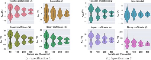
Figure A2. Uncertainty quantification of the estimated excitation profiles for INTC on 13 February 2018 under ${\text{Model}}_{\text{QI}}$. The parametric bootstrap procedure involves simulating 100 paths covering 2.5 hours of trading using the ML estimates of the parameters on the considered day and applying ML estimation again to each of the simulated paths. Three random sets of parameters are used as the initial guess in the optimisation procedure. We use the 100 estimates to compute a 99%-confidence interval for the truncated kernel norm (translucent area). The solid line corresponds to the ML estimates using the original INTC data.