Short-dated smile under rough volatility: asymptotics and numerics

Figures & data

Figure 1. Implied volatility smile approximations for the rBergomi model with parameters $\theta =1,{\sigma }_0=0.2,\eta =1.5,\rho =-0.7,H=0.3$, for expiry $t=0.05,0.2$. The Monte Carlo price is computed via the hybrid scheme for rBergomi in Bennedsen et al. (2017) with $\kappa =2$, with ${10}^9$ simulations and 500 time steps of length t/500. The rate function is computed using the Ritz method in Section 5.1 with N = 8 Haar basis functions, the coefficient $a\left(x\right)$ is computed using the Karhunen–Loeve decomposition with N = 300 Haar basis functions (KL). We also compare with $a\left(x\right)$ expanded at 0 ($a\left(x\right)\approx a\left(0\right)$).

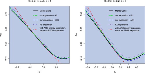
Figure 2. Implied volatility smile approximation for the rBergomi model with parameters ${\sigma }_0=0.15,\eta =1.8,\rho =-0.78,H=0.07$, for expiry t = 0.05. The Monte Carlo price is computed via the hybrid scheme for rBergomi in Bennedsen et al. (2017) with $\kappa =2$, with ${10}^9$ simulations and 500 time steps. The rate function is computed using the Ritz method with N = 9 Fourier basis functions.

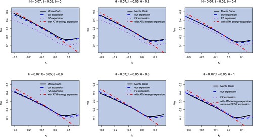
Figure 3. Implied volatility smile approximation for the rBergomi model with parameters $\theta =0,{\sigma }_0=0.15,\eta =1.8,\rho =-0.78,H=0.07$, for expiry t = 0.01, 0.05, 0.2. The Monte Carlo price is computed via the hybrid scheme for rBergomi in Bennedsen et al. (2017) with $\kappa =2$, with ${10}^9$ simulations and 500 time steps of length t/500. The rate function is computed using the Ritz method with N = 9 Fourier basis functions.

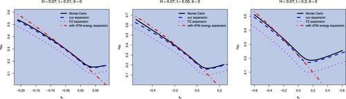
Figure 4. Term structure of volatility for the rBergomi model with parameters ${\sigma }_0=0.15,\eta =1.8,\rho =-0.78,H=0.3$ (above) and with parameters ${\sigma }_0=0.2557,\eta =0.2928,\rho =-0.7571,H=0.1$ (below). We plot ATM implied volatility as expiration time increases. We consider shorter expiries in the case of rougher trajectories (smaller Hurst parameter H; however, in this case we also take a smaller vol-of-vol parameter η). The Monte Carlo prices are computed via the hybrid scheme in Bennedsen et al. (2017) with $\kappa =2$, with ${10}^9$ simulations and 500 time steps.

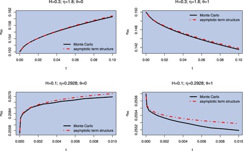
Figure 5. Moderate deviation with $\text{β}=0.06$ and x = 0.4 (time varying log-strike $k_t=x{t}^{1/2-H+\text{β}}$) of implied volatility in rBergomi model with ${\sigma }_0=0.2557,\eta =0.2928,\rho =-0.7571,H=0.1,\theta =0$. Simulation parameters: ${10}^8$ simulation paths, 500 time steps. Time interval $[0,0.1]$.

Bennedsen, M., Lunde, A. and Pakkanen, M.S., Hybrid scheme for Brownian semistationary processes. Finance Stoch., 2017, 21(4), 931–965.

 Web of Science ®Google Scholar