When do systematic strategies decay?

Figures & data

Table 1. Start dates of accounting and price data sets for different international indexes.

Index name	Start date
S&P/ASX 200 Index	2001-11-01
Bloomberg European 500	1999-01-01
Hang Seng Composite Index	2002-01-01
Korea Kospi Index	2003-12-01
Russell 3000 Index	1995-01-01
Russell 1000 Index	1995-01-01
China SE Shang Composite	2002-01-01
S&P/TSX Composite Index	2001-04-01
TOPIX 500 Index (TSE)	2007-01-01
FTSE 100 Index	1996-01-01

Table 2. Summary statistics on our sample of 72 factors. Annualised Sharpe ratio and t-stats were computed with monthly returns. All factors are beta-neutralised, computed on CRSP from 1963 to 2014.

	Entire sample		In-sample Sharpe $>0$		In-sample Sharpe $>0.3$
	Sharpe ratio	t-stat	Sharpe ratio	t-stat	Sharpe ratio	t-stat
Mean	0.98	4.52	1.02	4.73	1.15	5.34
Median	0.85	3.79	0.88	3.84	0.99	4.55
$Q_1$	0.43	1.89	0.46	1.98	0.69	2.75
$Q_3$	1.33	6.24	1.38	6.39	1.46	7.10
N	72		69		60

Figure 1. Left panel: Sharpe ratios of factors post-publication versus pre-publication. The regression is performed with OLS and has a $R^2$ of 67%. Observations are divided into deciles and we compute the average (resp. median) Sharpe ratio in-sample (resp. post-publication). The error bars show the standard deviation in the y direction. Right panel: Discount ratio versus pre-publication Sharpe ratio. The median discount ratio is 0.55.

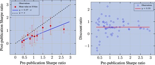
Figure 2. Raw and size-adjusted Sharpe ratios on liquidity pools vs. their original pool (as specified by the authors) counterparts. Observations are cut into five bins based on quantiles, we then compute the average (resp. median) Sharpe ratio on CRSP (resp. CRSP LQ 1000 or 500). Factors are beta-neutralised and Sharpe ratios below 0.3 on the entire CRSP universe (in-sample) are excluded.

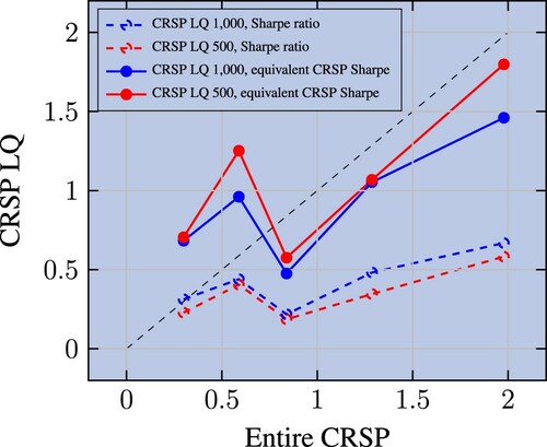
Table 3. Median discount ratio.

				Size adjusted
Country	Index/pool	Average size	Raw	Simple	Complex
Panel A: US pools
United States	CRSP post-publication	4694	0.55	0.52	0.54
United States	Russell 3000 Index	2933	0.20	0.26	0.22
United States	Russell 1000 Index	975	0.17	0.37	0.32
Panel B: Non-US pools
Australia	S&P/ASX 200 Index	200	0.08	0.38	1.00
Europe	Bloomberg European 500	505	0.09	0.24	0.37
Hong Kong	Hang Seng Composite Index	312	0.20	0.75	0.74
Korea	Korea Kospi Index	734	0.20	0.52	0.44
China	China SE Shanghai Composite	918	0.18	0.39	0.32
Canada	S&P/TSX Composite Index	244	0.11	0.47	0.87
Japan	TOPIX 500 Index (TSE)	500	−0.01	−0.02	0.32
United Kingdom	FTSE 100 Index	100	0.08	0.53	1.78
Average non-US		439	0.11	0.41	0.73

Table 4. Statistics for arbitrage variables before standardization. We only retain strategies with an in-sample Sharpe ratio on CRSP higher than 0.3.

	Mean	Median	$Q_1$	$Q_3$	$N$
log holding period	6.08	6.22	5.91	6.40	58
log mkt cap long short	0.88	0.62	−0.08	2.00	58
log mkt cap short	0.95	0.66	0.04	1.64	58
liquidity	−0.64	−0.74	−0.99	−0.17	58

Note: Log holding period is the natural logarithm of the factor's holding period. Log mkt cap long short is the natural logarithm of the ratio factor's market cap to average market cap. Log mkt cap short is defined as the natural logarithm of the ratio factor's short leg market cap to average market cap. Liquidity is the ratio of factor's liquidity (minus Amihud's liquidity) to average pool liquidity.

Figure 3. Number of Compustat fields (resp. operations) used to compute the factors' characteristic, as a function of publication date. We only show factors whose in-sample Sharpe ratio is greater than 0.3. One dot per factor. The red line represents a moving average of five factors.

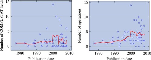
Figure 4. Distribution of in-sample Sharpe ratios of factors. We show original factors and a version where we remove the top 0.1% portfolio returns (Broderick et al. 2021). All 72 factors are beta-neutralised.

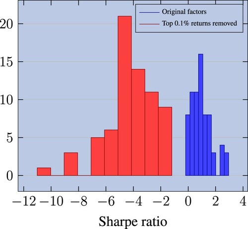
Table 5. Stats for overfitting variables before standardization. We only retain strategies with an in-sample Sharpe ratio on CRSP higher than 0.3.

	Mean	Median	$Q_1$	$Q_3$	$N$
dummy tstat	0.28	0.00	0.00	1.00	60
log q span cv	−1.95	−2.11	−2.43	−1.37	58
diff from best q	0.15	0.08	0.03	0.21	58
dummy nb fields	0.35	0.00	0.00	1.00	60
dummy nb operations	0.75	1.00	0.75	1.00	60
sqrt nb months is	−16.06	−16.57	−18.52	−12.64	60
log std subset	−3.41	−3.45	−3.82	−2.91	57
diff w drop data	5.42	5.35	4.34	6.42	58

Note: Dummy tstat equals 1 (resp. 0) if the factor's t-stat is less (resp. greater) than 3. Log q span cv is the natural logarithm of the coefficient of variation of the factor's SR when varying the top and bottom quantiles that defines long/short legs. Diff from best q is the difference between the maximal in-sample SR (by varying the quantiles) and the original in-sample SR. Dummy nb fields equals 1 (resp. 0) if the number of Compustat variables to define the factor is greater or equal (resp. less) than 2. Dummy nb operations equal 1 (resp. 0) if the number of operations to define the factor is greater or equal (resp. less) than 2. Sqrt nb months is minus the square root of number of months used in the back test of the factor. Log std subset is the natural logarithm of the standard deviation of SR when removing a random 10% of stocks. Diff w drop data is the difference between the original in-sample SR and the SR when removing the top 0.1% portfolio returns.

Figure 5. Left panel: discount ratio as a function of publication date. Factors are beta-neutralised and computed on CRSP and we only retain those with Sharpe ratio greater than 0.3; one dot per factor; the red line draws a linear trend, fitted on blue dots, where dates are represented in Unix time. Right panel: average PnL of factors, centered on publication date; the average PnL is detrended based on the pre-publication period; factors are market-neutralised and, to be comparable, risk-managed; we use with the original stock pool and eliminate strategies that do not replicate well in sample.

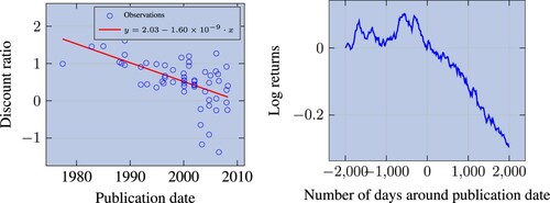
Table 6. OLS univariate regressions of the discount ratio on arbitrage variables (t-stats in parentheses).

	1	2	3	4
const	0.87	0.70***	0.72***	0.36***
	(1.22)	(7.8)	(7.86)	(2.64)
log holding period	−0.05
	(−0.41)
log mkt cap long short		−0.14**
		(−2.48)
log mkt cap short			−0.15***
			(−2.67)
liquidity				−0.34*
				(−1.95)
N	58	58	58	58
$R^2$	0.00	0.10	0.11	0.06

Note: ${}^{\ast \ast \ast }p<0.01$; ${}^{\ast \ast }p<0.05$; ${}^{\ast }p<0.1$

Table 7. OLS univariate regressions of the discount ratio on overfitting variables (t-stats in parentheses).

	1	2	3	4	5
const	0.59${}^{\ast \ast \ast }$	0.52${}^{\ast \ast \ast }$	0.54${}^{\ast \ast \ast }$	0.63${}^{\ast \ast \ast }$	0.92${}^{\ast \ast \ast }$
	(6.12)	(6.09)	(6.39)	(6.29)	(5.9)
dummy tstat	−0.15
	(−0.8)
log q span cv		−0.10
		(−1.08)
diff from best q			−0.07
			(−0.83)
dummy nb fields				−0.23
				(−1.37)
dummy nb operations					−0.49${}^{\ast \ast \ast }$
					(−2.72)
N	60	58	58	60	60
$R^2$	0.01	0.02	0.01	0.03	0.11
const	0.55${}^{\ast \ast \ast }$	0.59${}^{\ast \ast \ast }$	0.59${}^{\ast \ast \ast }$	0.53${}^{\ast \ast \ast }$
	(6.73)	(8.01)	(7.99)	(7.72)
sqrt nb months is	0.08
	(0.91)
log std subset		−0.16${}^{\ast \ast }$
		(−2.04)
diff w drop data			−0.21${}^{\ast \ast \ast }$
			(−2.99)
dapublished				−0.35${}^{\ast \ast \ast }$
				(−5.06)
N	60	57	58	60
$R^2$	0.01	0.07	0.14	0.31

Note: ${}^{\ast \ast \ast }p<0.01$; ${}^{\ast \ast }p<0.05$; ${}^{\ast }p<0.1$.

Table 8. OLS regressions with arbitrage and overfitting vulnerabilities.

	Discount ratio
Dependent variable:	1	2	3	4	5	6
Year of publication −1990	−.05${}^{\ast \ast \ast }$				−.041${}^{\ast \ast \ast }$	−.044${}^{\ast \ast \ast }$
	(−4.9)				(−4.9)	(−5.2)
Arbitrage vulnerability		−.28${}^{\ast \ast }$		−.21${}^{\ast \ast }$	−.13
		(−2.6)		(−2.1)	(−1.5)
Overfitting vulnerability			−.34${}^{\ast \ast \ast }$	−.28${}^{\ast \ast }$	−.28${}^{\ast \ast \ast }$	−.31${}^{\ast \ast \ast }$
			(−3.1)	(−2.5)	(−3)	(−3.5)
Constant	1${}^{\ast \ast \ast }$	.58${}^{\ast \ast \ast }$	.55${}^{\ast \ast \ast }$	.55${}^{\ast \ast \ast }$	.92${}^{\ast \ast \ast }$	.94${}^{\ast \ast \ast }$
	(8.7)	(7.7)	(7.4)	(7.7)	(9.6)	(9.8)
N	60	58	55	55	55	55
$R^2$	0.30	0.11	0.15	0.19	0.47	0.45

Note: ${}^{\ast \ast \ast }p<0.01$; ${}^{\ast \ast }p<0.05$; ${}^{\ast }p<0.1$.

Table A1. List of factors and the corresponding references.

Factor	Reference article
Price earnings	Basu (1977)
Unexpected quarterly earnings	Rendleman et al. (1982)
Long term reversal	De Bondt and Thaler (1985)
Debt equity	Bhandari (1988)
Change in inventory-to-assets	Ou and Penman (1989)
Change in dividend per share	Ou and Penman (1989)
Change in capital expenditures-to-assets	Ou and Penman (1989)
Return on total assets	Ou and Penman (1989)
Debt repayment	Ou and Penman (1989)
Depreciation-to-PP&E	Holthausen and Larcker (1992)
Change in depreciation-to-PP&E	Holthausen and Larcker (1992)
Change in total assets	Holthausen and Larcker (1992)
Size	Fama and French (1993)
Book-to-market	Fama and French (1993)
Momentum	Jegadeesh and Titman (1993)
Sales growth	Lakonishok et al. (1994)
Cash flow-to-price	Lakonishok et al. (1994)
Working capital accruals	Sloan (1996)
Sales-to-price	Barbee et al. (1996)
Share turnover	Haugen and Baker (1996)
Cash flow-to-price variability	Haugen and Baker (1996)
Trading volume trend	Haugen and Baker (1996)
Inventory	Abarbanell and Bushee (1998)
Gross margin	Abarbanell and Bushee (1998)
Capital expenditures	Abarbanell and Bushee (1998)
Industry momentum	Moskowitz and Grinblatt (1999)
F-score	Piotroski (2000)
Industry adjusted book-to-market	Asness et al. (2000)
Industry adjusted cash flow-to-price	Asness et al. (2000)
Industry adjusted size	Asness et al. (2000)
Industry adjusted momentum	Asness et al. (2000)
Industry adjusted long term reversal	Asness et al. (2000)
Industry adjusted short term reversal	Asness et al. (2000)
Dollar volume	Chordia et al. (2001)
Dollar volume coefficient of variation	Chordia et al. (2001)
Share turnover coefficient of variation	Chordia et al. (2001)
Change in inventory	Thomas and Zhang (2002)
Change in current assets	Thomas and Zhang (2002)
Depreciation	Thomas and Zhang (2002)
Change in accounts receivable	Thomas and Zhang (2002)
Other accruals	Thomas and Zhang (2002)
Illiquidity	Amihud (2002)
Liquidity	Pástor and Stambaugh (2003)
Idiosyncratic return volatility x book-to-market	Ali et al. (2003)
Price x book-to-market	Ali et al. (2003)
Operating cash flow-to-price	Desai et al. (2004)
Abnormal corporate investment	Titman et al. (2004)
Accrual quality	Francis et al. (2004)
Earnings persistence	Francis et al. (2004)
Smoothness	Francis et al. (2004)
Value relevance	Francis et al. (2004)
Timeliness	Francis et al. (2004)
Tax income-to-book income	Lev and Nissim (2004)
Price delay	Hou and Moskowitz (2005)
Firm age	Jiang et al. (2005)
Duration	Jiang et al. (2005)
Change in current operating assets	Richardson et al. (2005)
Change in non-current operating liabilities	Richardson et al. (2005)
Growth in capital expenditures	Anderson and Garcia-Feijoo (2006)
Growth in capital expenditures (alternative)	Anderson and Garcia-Feijoo (2006)
Low volatility	Ang et al. (2006)
Low beta ΔVIX	Ang et al. (2006)
Zero trading days	Liu (2006)
Composite issuance	Daniel and Titman (2006)
Intangible return	Daniel and Titman (2006)
Earnings surprises x revenue surprises	Jegadeesh and Livnat (2006)
Industry concentration	Hou and Robinson (2006)
Change in shares outstanding	Pontiff and Woodgate (2008)
Seasonality	Heston and Sadka (2008)
Investment	Lyandres et al. (2008)
Investment growth	Xing (2007)
Change in asset turnover	Soliman (2008)

Table A2. OLS regressions of equivalent Sharpe ratio of CRSP LQ 500 (resp. 1000) on CRSP (t-stats in parenthesis).

	CRSP LQ 500	CRSP LQ 1000
coef	0.80${}^{\ast \ast \ast }$	0.67${}^{\ast \ast \ast }$
	(8.68)	(8.52)
N	60	60
$R^2$	0.56	0.55

Note: ${}^{\ast \ast \ast }p<0.01$; ${}^{\ast \ast }p<0.05$; ${}^{\ast }p<\mathrm{0.1.}$

Table A3. Correlation matrix for arbitrage variables.

	log holding period	log mkt cap long short	log mkt cap short	liquidity
log holding period	1.00
log mkt cap long short	−0.23	1.00
log mkt cap short	−0.08	0.89	1.00
liquidity	−0.07	0.78	0.62	1.00

Table A4. Correlation matrix for overfitting variables; dts = dummy tstat, lqscv = log q span cv, dbq = diff from best q, dnf = dumy nb fields, dno = dummy nb operations, snm = sqrt nb months is, lss = log std subset, ddd = diff w drop data.

	dts	lqscv	dbq	dnf	dno	snm	lss	ddd	dp
dts	1.00
lqscv	0.58	1.00
dbq	0.03	0.16	1.00
dnf	0.13	0.06	−0.02	1.00
dno	0.03	−0.07	0.06	0.23	1.00
snm	0.26	−0.05	−0.09	0.22	0.17	1.00
lss	0.14	0.16	0.00	0.44	0.43	0.48	1.00
ddd	−0.05	0.05	−0.05	0.24	0.35	0.22	0.48	1.00
dp	−0.11	0.14	0.09	0.09	0.29	−0.54	−0.04	0.27	1.00

Figure A1. Number of constituents in each pool.

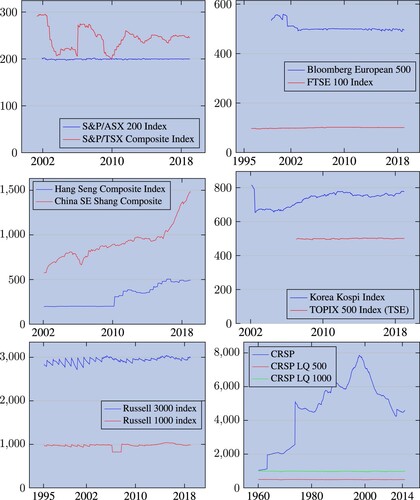
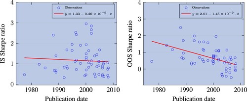
Figure A2. In-sample (resp. out-of-sample) Sharpe ratio as a function of publication date. Factors are beta-neutralised and computed on CRSP, conditional on its in-sample Sharpe ratio being greater than 0.3. One dot per factor. The red line draws a linear trend, fitted on blue dots, where dates are represented in Unix time. The $R^2$ are 0.4% and 24% respectively.

Broderick, T., Giordano, R. and Meager, R., An automatic finite-sample robustness metric: When can dropping a little data make a big difference? 2021, arXiv preprint. https://arxiv.org/abs/2011.14999.

 Google Scholar

Basu, S., Investment performance of common stocks in relation to their price-earnings ratios: A test of the efficient market hypothesis. J. Finance, 1977, 32(3), 663–682. doi:10.1111/j.1540-6261.1977.tb01979.x

 Web of Science ®Google Scholar

Rendleman, R.J., Jones, C.P. and Latané, H.A., Empirical anomalies based on unexpected earnings and the importance of risk adjustments. J. Financ. Econ., 1982, 10(3), 269–287. doi:10.1016/0304-405X(82)90003-4

 Web of Science ®Google Scholar

De Bondt, W.F.M. and Thaler, R., Does the stock market overreact?. J. Finance, 1985, 40(3), 793–805. doi:10.1111/j.1540-6261.1985.tb05004.x

 Web of Science ®Google Scholar

Bhandari, L.C., Debt/equity ratio and expected common stock returns: Empirical evidence. J. Finance, 1988, 43(2), 507–528. doi:10.1111/j.1540-6261.1988.tb03952.x

 Web of Science ®Google Scholar

Ou, J.A. and Penman, S.H., Financial statement analysis and the prediction of stock returns. J. Accounting Econ., 1989, 11, 295–329. doi:10.1016/0165-4101(89)90017-7

 Web of Science ®Google Scholar

Holthausen, R.W. and Larcker, D.F., The prediction of stock returns using financial statement information. J. Accounting Econ., 1992, 15, 373–411. doi:10.1016/0165-4101(92)90025-W

 Web of Science ®Google Scholar

Fama, E.F. and French, K.R., Common risk factors in the returns on stocks and bonds. J. Financ. Econ., 1993, 33(1), 3–56. doi:10.1016/0304-405X(93)90023-5

 Web of Science ®Google Scholar

Jegadeesh, N. and Titman, S., Returns to buying winners and selling losers: Implications for stock market efficiency. J. Finance, 1993, 48(1), 65–91. doi:10.2307/2328882

 Web of Science ®Google Scholar

Lakonishok, J., Shleifer, A. and Vishny, R.W., Contrarian investment, extrapolation, and risk. J. Finance, 1994, 49(5), 1541–1578. doi:10.1111/j.1540-6261.1994.tb04772.x

 Web of Science ®Google Scholar

Sloan, R.G., Do stock prices fully reflect information in accruals and cash flows about future earnings? Account Rev., 1996, 71(3), 289–315. http://www.jstor.org/stable/248290.

 Web of Science ®Google Scholar

Barbee, W.C., Mukherji, S and Raines, G.A., Do sales–price and debt–equity explain stock returns better than book–market and firm size? Financ. Anal. J., 1996, 52(2), 56–60. doi:10.2469/faj.v52.n2.1980

 Google Scholar

Haugen, R.A. and Baker, N.L., Commonality in the determinants of expected stock returns. J. Financ. Econ., 1996, 41(3), 401–439. doi:10.1016/0304-405X(95)00868-F

 Web of Science ®Google Scholar

Abarbanell, J.S. and Bushee, B.J., Abnormal returns to a fundamental analysis strategy. Account Rev., 1998, 73(1), 19–45. http://www.jstor.org/stable/248340.

 Web of Science ®Google Scholar

Moskowitz, T.J. and Grinblatt, M., Do industries explain momentum? J. Finance, 1999, 54(4), 1249–1290. doi:10.1111/0022-1082.00146

 Web of Science ®Google Scholar

Piotroski, J.D., Value investing: The use of historical financial statement information to separate winners from losers. J. Accounting Res., 2000, 38, 1–41. doi:10.2307/2672906

 Web of Science ®Google Scholar

Asness, C.S., Porter, R.B. and Stevens, R.L., Predicting stock returns using industry-relative firm characteristics. 2000. doi:10.2139/ssrn.213872.

 Google Scholar

Chordia, T., Subrahmanyam, A. and Anshuman, V., Trading activity and expected stock returns. J. Financ. Econ., 2001, 59(1), 3–32. doi:10.1016/S0304-405X(00)00080-5

 Web of Science ®Google Scholar

Thomas, J.K. and Zhang, H., Inventory changes and future returns. Rev. Account. Stud., 2002, 7, 163–187. doi:10.1023/A:1020221918065

 Google Scholar

Amihud, Y., Illiquidity and stock returns: Cross-section and time-series effects. J. Financ. Markets, 2002, 5(1), 31–56. doi:10.1016/S1386-4181(01)00024-6

 Web of Science ®Google Scholar

Pástor, L. and Stambaugh, R.F., Liquidity risk and expected stock returns. J. Polit. Econ., 2003, 111(3), 642–685. doi:10.1086/374184

 Web of Science ®Google Scholar

Ali, A., Hwang, L.S. and Trombley, M.A., Arbitrage risk and the book-to-market anomaly. J. Financ. Econ., 2003, 69(2), 355–373. doi:10.1016/S0304-405X(03)00116-8

 Web of Science ®Google Scholar

Desai, H., Rajgopal, S. and Venkatachalam, M., Value–Glamour and accruals mispricing: One anomaly or two? Accounting Rev., 2004, 79(2), 355–385. doi:10.2308/accr.2004.79.2.355

 Web of Science ®Google Scholar

Titman, S., Wei, K.C.J. and Xie, F., Capital investments and stock returns. J. Finan. Quant. Anal., 2004, 39(4), 677–700. doi:10.1017/S0022109000003173

 Web of Science ®Google Scholar

Francis, J., LaFond, R., Olsson, P.M. and Schipper, K., Costs of equity and earnings attributes. Accounting Rev., 2004, 79(4), 967–1010. doi:10.2308/accr.2004.79.4.967

 Web of Science ®Google Scholar

Lev, B. and Nissim, D., Taxable income, future earnings, and equity values. Accounting Rev., 2004, 79(4), 1039–1074. doi:10.2308/accr.2004.79.4.1039

 Web of Science ®Google Scholar

Hou, K. and Moskowitz, T.J., Market frictions, price delay, and the cross-section of expected returns. Rev. Financ. Stud., 2005, 18(3), 981–1020. doi:10.1093/rfs/hhi023

 Web of Science ®Google Scholar

Jiang, G., Lee, C.M.C. and Zhang, Y., Information uncertainty and expected returns. Rev. Accounting Stud., 2005, 10, 185–221. doi:10.1007/s11142-005-1528-2

 Web of Science ®Google Scholar

Richardson, S.A., Sloan, R.G., Soliman, M.T. and Tuna, I., Accrual reliability, earnings persistence and stock prices. J. Accounting Econ., 2005, 39(3), 437–485. doi:10.1016/j.jacceco.2005.04.005

 Web of Science ®Google Scholar

Anderson, C.W. and Garcia-Feijoo, L., Empirical evidence on capital investment, growth options, and security returns. J. Finance, 2006, 61(1), 171–194. doi:10.1111/j.1540-6261.2006.00833.x

 Web of Science ®Google Scholar

Ang, A, Hodrick, R.J., Xing, Y. and Zhang, X., The cross-section of volatility and expected returns. J. Finance, 2006, 61(1), 259–299. doi:10.1111/j.1540-6261.2006.00836.x

 Web of Science ®Google Scholar

Liu, W., A liquidity-augmented capital asset pricing model. J. Financ. Econ., 2006, 82(3), 631–671. doi:10.1016/j.jfineco.2005.10.001

 Web of Science ®Google Scholar

Daniel, K. and Titman, S., Market reactions to tangible and intangible information. J. Finance, 2006, 61(4), 1605–1643.doi:10.1111/j.1540-6261.2006.00884.x

 Web of Science ®Google Scholar

Jegadeesh, N. and Livnat, J., Revenue surprises and stock returns. J. Accounting Econ., 2006, 41(1), 147–171. doi:10.1016/j.jacceco.2005.10.003

 Web of Science ®Google Scholar

Hou, K. and Robinson, D.T., Industry concentration and average stock returns. J. Finance, 2006, 61(4), 1927–1956. doi:10.1111/j.1540-6261.2006.00893.x

 Web of Science ®Google Scholar

Pontiff, J. and Woodgate, A., Share issuance and cross-sectional returns. J. Finance, 2008, 63(2), 921–945. doi:10.1111/j.1540-6261.2008.01335.x

 Web of Science ®Google Scholar

Heston, S.L. and Sadka, R., Seasonality in the cross-section of stock returns. J. Financ. Econ., 2008, 87(2), 418–445. doi:10.1016/j.jfineco.2007.02.003

 Web of Science ®Google Scholar

Lyandres, E., Sun, L. and Zhang, L., The new issues puzzle: Testing the investment-based explanation. Rev. Financ. Stud., 2008, 21(6), 2825–2855. doi:10.1093/rfs/hhm058

 Web of Science ®Google Scholar

Xing, Y., Interpreting the value effect through the Q-theory: An empirical investigation. Rev. Financ. Stud., 2007, 21(4), 1767–1795. doi:10.1093/rfs/hhm051

 Web of Science ®Google Scholar

Soliman, M.T., The use of dupont analysis by market participants. Account. Rev., 2008, 83(3), 823–853. doi:10.2308/accr.2008.83.3.823

 Web of Science ®Google Scholar