Asymmetric short-rate model without lower bound

Figures & data

Figure 1. Interpolated caplet prices and market-implied probability density under ${\mathbb{Q}}^S$ constructed based on the cap market data (quoted in normal volatility) on March 31, 2016. Panel (a) gives the market caplet prices (dots) computed by the Bachelier formula alongside with interpolated price curve obtained by the no-arbitrage cubic spline smoothing technique. Panel (b) provides the $L(6M,1Y)$ forward rate density implied from the interpolated caplet prices using equation (25(25) $\begin{array}{r}{f}_{L(T,S)|{\mathcal{F}}_t}^S\left(K\right)=\frac{\frac{{\mathrm{\partial }}^2}{\mathrm{\partial }{K}^2}{\mathrm{C}\mathrm{p}\mathrm{l}}_t(T,S,K)}{\mathrm{\Delta }{P}_t\left(S\right)}.\end{array}$(25) ). (a) Interpolated price curve and (b) implied density of $L(6M,1Y)$.

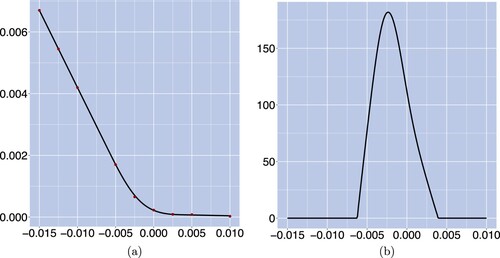
Figure 2. Implied-volatility curves with associated squared errors (in bps) and relative volatility errors on March 31, 2016, where the models are calibrated on the criteria of implied volatility error minimization. Panel (a) shows the implied-volatility curves with respect to the strike for the market (dashed), Hull–White (□), CIR++ ($\mathrm{△}$) and VaCIR++ (⋄) models. Panel (b) and Panel (c) provide respectively the box plots of the associated squared and relative errors for the three candidate models. (a) Implied-volatility curve; (b) implied vol squared error and (c) implied vol relative error.

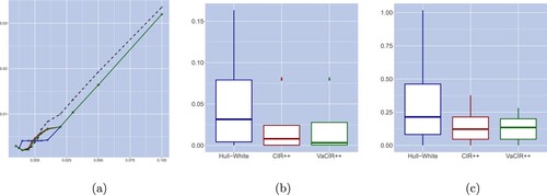
Figure 3. Caplet price curves with corresponding squared errors (in bps) and relative pricing errors on March 31, 2016, where models are calibrated on the criteria of implied volatility error minimization. Panel (a) displays the market and modelled caplet prices with respect to the strike for the market (dashed), Hull–White (□), CIR++ ($\mathrm{△}$) and VaCIR++ (⋄) models. Panel (b) and panel (c) provide respectively the box plots of the corresponding squared errors and relative errors for the three candidate models. (a) Caplet price curve, (b) price squared error and (c) price relative error.

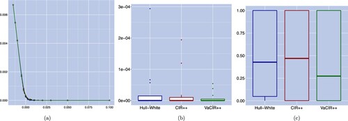
Figure 4. Density curves of the forward rate $L(6M,1Y)$ on March 31, 2016, where models are calibrated on the criteria of implied volatility error minimization. Panel (a), panel (b) and panel (c) exhibit the market-implied forward density curve and the modelled forward density curves (dashed lines) and under the Hull–White, the CIR++ and VaCIR++ models, respectively (solid lines). (a) Hull–White model, (b) CIR++ model and (c) VaCIR++ model.

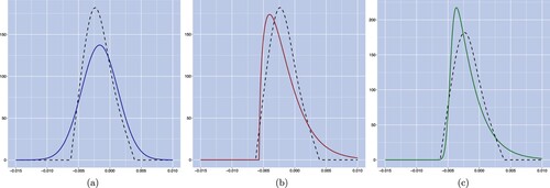
Figure 5. Density curves of the forward rate $L(6M,1Y)$ on March 31, 2016, where models are calibrated on the criteria of JS divergence minimization. Panel (a), panel (b) and panel (c) exhibit the market-implied forward density curve (dashed lines) and the modelled forward density curves under the Hull–White, CIR++ and VaCIR++ models, respectively (solid lines). (a) Hull–White model, (b) CIR++ model and (c) VaCIR++ model.

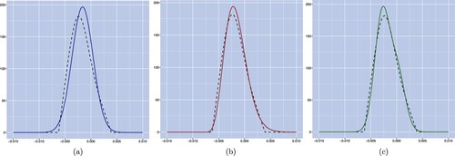
Figure 6. Caplet price curves with corresponding mean squared errors (in bps) and relative pricing errors on March 31, 2016, where models are calibrated on the criteria of JS divergence minimization. Panel (a) displays the market and modelled caplet prices with respect to the strike for the market (dashed), Hull–White (□), CIR++ ($\mathrm{△}$) and VaCIR++ (⋄) models. Panel (b) and panel (c) provide respectively the box plots of the corresponding mean squared errors and relative errors for the three candidate models. (a) Caplet price curve, (b) price squared error and (c) price relative error.

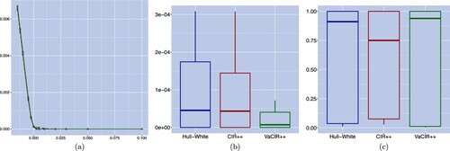
Figure 7. Implied-volatility curves with associated squared and relative volatility errors on March 31, 2016, where the models are calibrated on the criteria of JS divergence minimization. Panel (a) contains the implied-volatility curves with respect to the strike for the market (dashed), Hull–White (□), CIR++ ($\mathrm{△}$) and VaCIR++ (⋄) models. Panel (b) and Panel (c) provide respectively the box plots of the associated squared errors and relative errors for the three candidate models. (a) Implied-volatility curve; (b) implied vol squared error and (c) implied vol relative error.

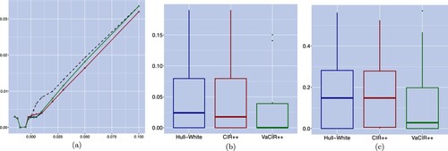
Figure 8. Density curves of the forward rate $L(6M,1Y)$ on March 31, 2016, where models are calibrated on the criteria of JS divergence minimization. Panel (a), Panel (b) and panel (c) exhibit the market-implied forward density curve and the modelled forward density curves (dashed lines) and under the G2++, CIR2++ and VaCIR++ models, respectively (solid lines). (a) The G2++ model; (b) the CIR2++ model and (c) VaCIR++ model.

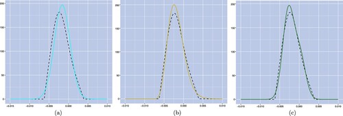
Figure 9. Evolution over time of the JS divergence resulting from the density matching calibration under the Hull–White (□, dark blue), CIR++ ($\mathrm{△}$, red), G2++ (♦, light blue), CIR2++ (+, yellow) and VaCIR++ ($◊$, green) models.

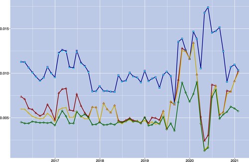
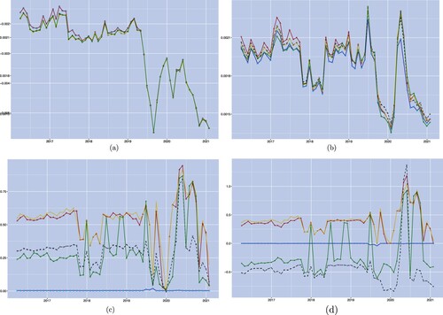
Figure 10. Time series of the $L(6M,1Y)$ conditional moments for the market (°) and for the Hull–White (□, dark blue), CIR++ ($\mathrm{△}$, red), G2++ (♦, light blue), CIR2++ (+, yellow) and VaCIR++ ($◊$, green) models. (a) Conditional mean; (b) conditional standard deviation; (c) conditional skewness and (d) conditional excess kurtosis.