Leveraged funds: robust replication and performance evaluation

Figures & data

Figure 1. Buy (dashed) and sell (solid) boundaries (vertical, as risky weights π) versus average tracking error $\text{TrE}$ (horizontal) for leveraged (top) and inverse (bottom) funds, with multipliers 4 (top), 3, 2, $-1$, $-2$, $-3$ (bottom). As aversion to tracking error γ decreases from left ($\approx {10}^6$) to right ($\approx {10}^{-4}$), for inverse funds (bottom) the trading boundaries widen around the target, whereas for leveraged funds (top) they first widen and then collapse to one. $ϵ=1\mathrm{\%}$ and zero risk premium.

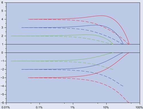
Figure 2. Negative tracking difference ($-\text{TrD}$, vertical) against tracking error (horizontal) for leveraged (solid) and inverse (dashed) funds, in logarithmic scale, from −3, +4 (top), to −2, +3 (middle), and −1, +2 (bottom). As aversion to tracking error γ decreases from left ($\approx {10}^6$) to right ($\approx {10}^{-4}$), a k + 1-leveraged fund is akin to a $-k$ inverse one, as the respective curves (same color) approach low and high $\text{TrE}$ aversion. $ϵ=1\mathrm{\%}$, $\sigma =16\mathrm{\%}$, and zero risk premium.

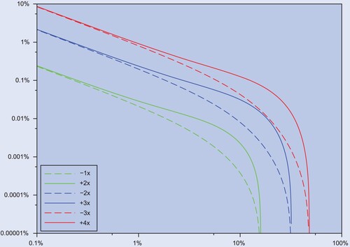
Figure 3. Exact $R^2$ (vertical) for inverse and leveraged factors Λ (horizontal), with aversion parameter $\gamma =0.5$ (blue) and $\gamma =1$ (green).

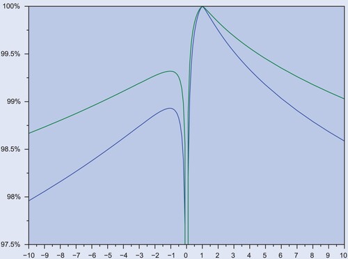
Table 1. Average exposure (left) and average daily turnover (right), both as percent of funds' values, in different asset classes for S&P 500 LIETFs: SPXU (−3), SDS (−2), SH (−1), SSO (+2), UPRO (+3), from 2018-01-26 to 2018-04-06.

Factor	Futures	Stocks	Index Swaps	Factor	Futures	Stocks	Index Swaps
−3.00	−12.45	0.00	−288.67	−3.00	2.96	0.00	10.65
−2.00	−9.85	0.00	−190.81	−2.00	1.60	0.00	5.24
−1.00	−5.18	0.00	−95.15	−1.00	0.82	0.00	2.37
2.00	5.90	83.20	110.89	2.00	0.84	0.46	1.77
3.00	6.90	83.93	209.16	3.00	1.17	0.78	5.89

Table 2. Summary statistics for the ratio (as percent) between (i) daily volume generated by LIETFs on the S&P 500 and (ii) daily volume in the S&P 500 components. Data from 2009-06-23 to 2018-03-27.

1% Quantile	Median	99% Quantile	Mean
0.01	0.15	0.86	0.20

Table 3. Performance of LIETFs on selected indexes through December $31st$, 2022. For each index, observations begin on the earliest date for which all inverse (−3, −2, −1) and leveraged (2, 3) multiples are available. (Earliest date is November $19th$, 2008.) Historical prices from Yahoo Finance, Interest rates from US Treasury.

Index	Ticker	X	Track. Error (bp)	Tracking Diff. (%)	Tracking Diff. (Gross) (%)	Implied Spread (bp)	Implied Spread (Gross) (bp)	Beta	T-stat (Beta) (%)	Vol. (%)	Years Data
	SPXU	−3	5.41	−1.18	−0.26	0.57	0.13	−2.99	4.00	52.59	13.51
S&P	SDS	−2	2.94	−0.74	0.15	0.77	−0.16	−2.00	−2.66	35.26	13.51
500	SH	−1	1.96	−0.68	0.21	4.24	−1.31	−1.01	−6.52	17.73	13.51
(SPY)	SSO	2	2.93	−1.59	−0.70	14.92	6.59	2.01	3.42	35.28	13.51
	UPRO	3	5.31	−2.29	−1.34	4.31	2.52	3.00	0.88	52.85	13.51
S&P	SMDD	−3	16.45	−2.45	−1.50	2.19	1.34	−2.96	5.10	61.90	12.88
Midcap	MZZ	−2	11.16	−2.31	−1.36	5.61	3.30	−1.94	11.75	40.54	12.88
400	MYY	−1	4.69	−1.11	−0.16	10.18	1.46	−1.00	1.89	20.76	12.88
(MDY)	MVV	2	4.22	−1.42	−0.47	11.78	3.92	1.99	−3.78	41.26	12.88
	UMDD	3	13.73	−1.58	−0.63	4.72	1.88	2.92	−12.06	60.88	12.88
MSCI	EDZ	−3	6.75	−1.39	−0.44	0.39	0.12	−2.96	13.31	66.89	13.57
Emerging	EEV	−2	4.51	−1.63	−0.68	1.23	0.51	−1.99	3.22	45.05	13.57
Markets	EUM	−1	2.83	−1.14	−0.19	4.87	0.81	−1.00	2.98	22.53	13.57
(EEM)	EET	2	12.26	−2.74	−1.79	50.78	33.20	1.95	−8.81	44.61	13.57
	EDC	3	7.74	−5.12	−4.18	6.65	5.42	2.93	−19.07	66.35	13.57
	SQQQ	−3	5.81	−2.28	−1.33	0.71	0.41	−2.96	14.15	61.63	12.88
Nasdaq	QID	−2	3.05	−1.21	−0.26	0.79	0.17	−1.99	5.39	41.45	12.88
100	PSQ	−1	2.13	−1.00	−0.05	4.10	0.20	−1.00	3.90	20.74	12.88
(QQQ)	QLD	2	3.06	−1.66	−0.71	9.75	4.16	1.99	−4.38	41.48	12.88
	TQQQ	3	5.43	−2.24	−1.30	2.61	1.51	2.95	−17.84	61.47	12.88
	TZA	−3	6.55	−4.95	−4.00	1.09	0.88	−2.99	5.10	72.59	14.11
Russell	TWM	−2	4.79	−3.12	−2.18	2.01	1.40	−1.99	5.47	48.37	14.11
2000	RWM	−1	2.66	−1.61	−0.67	5.20	2.14	−1.00	−1.80	24.37	14.11
(IWM)	UWM	2	4.47	−1.67	−0.67	9.03	3.62	1.99	−3.77	48.45	14.11
	TNA	3	6.03	−3.33	−2.38	2.70	1.93	2.96	−15.29	71.99	14.11
Barclays	TTT	−3	11.75	−2.13	−1.18	4.01	2.22	−2.87	15.84	41.88	10.75
20+	TBT	−2	8.90	−1.66	−0.74	9.43	4.20	−1.90	16.46	27.79	10.75
Treasury	TBF	−1	5.08	−1.24	−0.31	36.24	9.03	−0.96	12.38	14.05	10.75
(TLT)	UBT	2	11.07	−1.07	−0.12	68.49	7.95	1.93	−9.49	28.40	10.75
	TMF	3	5.87	−1.71	−0.76	6.44	2.87	2.94	−13.53	42.61	10.75
Dow Jones	SDOW	−3	4.61	−1.39	−0.45	0.61	0.19	−2.97	12.03	51.04	12.88
Industrial	DXD	−2	2.66	−0.92	0.03	0.93	−0.03	−1.99	6.84	34.20	12.88
Average	DOG	−1	1.77	−0.85	0.10	5.14	−0.59	−1.00	4.18	17.13	12.88
(DIA)	DDM	2	3.01	−1.58	−0.63	16.28	6.50	1.98	−10.35	34.08	12.88
	UDOW	3	5.48	−1.91	−0.96	3.96	1.99	2.95	−14.49	50.83	12.88

Table 4. Average exposure ($\overline{\text{β}}$) for typical factors (Λ) across trading costs (ε) and $\text{TrE}$ aversion (γ), obtained from equation (22(22) $\begin{array}{r}\overline{\text{β}}=\mathrm{\Lambda }-\frac{2\mathrm{\Lambda }-1}{\gamma }{\left(\frac{\gamma \mathrm{\Lambda }(\mathrm{\Lambda }-1)}{6}\right)}^{1/3}{ϵ}^{2/3}+O\left(ϵ\right)\end{array}$(22) ).

$ϵ=0.1\mathrm{\%}$
	γ
Λ	1	5	10
−3	−2.91	−2.97	−2.98
−2	−1.95	−1.98	−1.99
−1	−0.98	−0.99	−1.00
2	1.98	1.99	2.00
3	2.95	2.98	2.99
$ϵ=0.5\mathrm{\%}$
	γ
Λ	1	5	10
−3	−2.74	−2.91	−2.94
−2	−1.85	−1.95	−1.97
−1	−0.94	−0.98	−0.99
2	1.94	1.98	1.99
3	2.85	2.95	2.97

Figure 4. Trading boundaries (vertical) for factor $+3$ against tracking error (horizontal), from first-order asymptotics (25(25) $\begin{array}{rl}{\pi }_{\pm }& =\mathrm{\Lambda }\pm {\left(\frac{3}{4\gamma }{\mathrm{\Lambda }}^2\right(\mathrm{\Lambda }-1{)}^2)}^{1/3}{ϵ}^{1/3}\\ & -\frac{(\mathrm{\Lambda }-\kappa )}{\gamma }{\left(\frac{\gamma \mathrm{\Lambda }(\mathrm{\Lambda }-1)}{6}\right)}^{1/3}{ϵ}^{2/3}+O\left(ϵ\right).\end{array}$(25) ) (red) and exact solutions for $\kappa ={\mu }_t/{\sigma }_t^2=0$ (black), $\kappa =1.5625$ (blue), and $\kappa =3.125$ (green). For realistic levels of tracking error, the impact of κ is of second order.

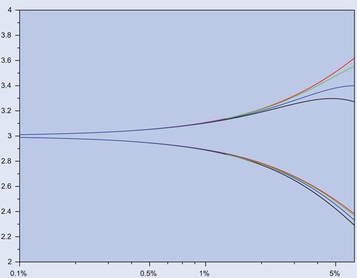
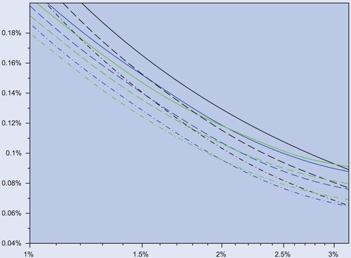
Figure 5. Negative tracking difference ($-\text{TrD}$) for $+3$ leveraged fund (vertical, colored solid lines) and $-2$ (dashed colored lines), against tracking error (TrE) (horizontal), for $\kappa ={\mu }_t/{\sigma }_t^2=0\mathrm{\%}$ (black), $\kappa =1.5625$ (blue) and $\kappa =3.125$ (green). The solid red line represents the asymptotic formula in (1(1) $\begin{array}{r}\widetilde{ϵ}:=\frac{12}{\sqrt{3}}\frac{(-\text{TrD})\cdot \text{TrE}}{{\overline{\sigma }}^3{\mathrm{\Lambda }}^2(1-\mathrm{\Lambda }{)}^2}.\end{array}$(1) ), which is the same for L and 1−L.

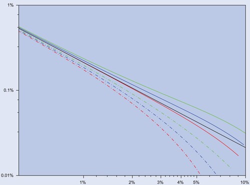
Figure 6. Negative tracking difference ($-\text{TrD}$) for a $+3$ leveraged fund (vertical), against tracking error (horizontal), for ${\mu }_t/{\sigma }_t=0$ (solid lines), 1.5625 (dashed) and 3.125 (dashed-dotted), when $ϵ=0.1\mathrm{\%}$. The black lines depicts the exact performance from (26(26) $\begin{array}{r}\underset{\phi \in \mathrm{\Phi }}{min}\text{EER}\left(\phi \right)=\frac{\gamma {\overline{\sigma }}^2}{2}({\pi }_{-}-\mathrm{\Lambda }{)}^2,\end{array}$(26) ) with $\overline{\sigma }=16\mathrm{\%}$. The blue and green lines correspond to Monte Carlo Estimates (15000 paths, daily grid) for the Black–Scholes (blue) and Heston (green) models, with time horizon of T = 5 years, daily sampling and trading frequency, and correlation $\rho =-0.9$.

Data Availability Statement

The code and data supporting this paper's findings are at https://github.com/guasoni/leveraged-funds.