Narrative triggers of information sensitivity

Figures & data

Table 1. Information sensitivity states of companies.

Panel A	Variable	Mean	SD	N	Share %
Trending for other	CDS spread	72.9	34.9	$941001$	48.9
	Google searches	36.1	22.9	$941001$	48.9
Insensitive state	CDS spread	101.7	64.0	$331201$	17.2
	Google searches	0	0.1	$331201$	17.2
Default state	CDS spread	3259.5	3500.7	$75916$	3.9
	Google searches	14.5	18.5	$75916$	3.9
Sensitive state	CDS spread	307.5	178.4	$575884$	29.9
	Google searches	28.9	22.9	$575884$	29.9
Panel B	Trending for other${}_{t-1}$	Insensitive state${}_{t-1}$	Default state${}_{t-1}$	Sensitive state${}_{t-1}$	Total share %
Trending for other${}_t$	90.986	8.525	0	0.463	100
Insensitive state${}_t$	24.22	69.076	0	6.661	100
Default state${}_t$	0	0	97.946	2.022	100
Sensitive state${}_t$	0.747	3.836	0.267	95.123	100

Figure 1. Information sensitivity states and CDS spreads for non-financial firms.

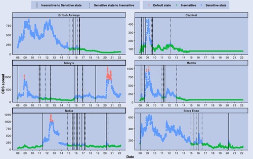
Figure 2. Information sensitivity states and CDS spreads for financial firms.

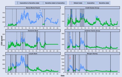
Figure 3. The evolution of the number of information sensitive companies in time.

Note: The following events are displayed with vertical lines. FED emergency meeting in March 14th, 2008: The Federal Reserve board had an emergency weekend meeting regarding Bear Stearns. Lehman Bankruptcy in September 15th, 2008: Lehman Brothers filed for bankruptcy. Greek election in June 17th, 2012: The centre-right wins legislative elections in Greece. Draghi Speech in July 26th, 2012: ECB president Mario Draghi gives the famous ‘the ECB is ready to do whatever it takes to preserve the euro’ - speech. COVID-19 in February 11th, 2020: WHO names the new virus as COVID-19.

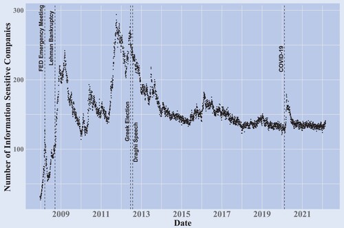
Figure 4. Hierarchical clustering of topics. The dendrogram plots the result of a hierarchical clustering model estimated with the topic word-distributions.

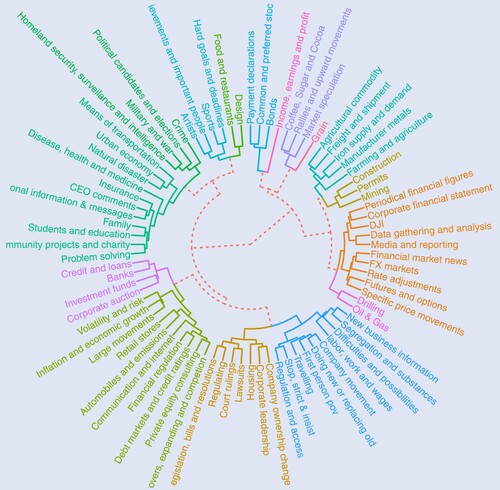
Figure 5. Prevalence of news topics in Time. The figure plots the topic distributions of each topic k aggregated to a monthly level across the period 1890–2022.

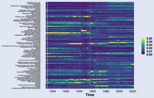
Figure 6. Evolution of unexpected news in selected topics. The figure plots the unpredictable part of topic's daily prevalence for each topic aggregated to a monthly level across the period 2006–2022.

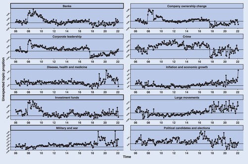
Figure 7. Evolution of unexpected news in time. The figure plots the unpredictable part of topic's daily prevalence for each topic k aggregated to a monthly level across the period 2006–2022.

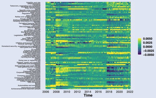
Figure 8. Distribution of the primordial - conceptual word share difference across authors. A total amount of 3062 authors and 74 articles per author on average. (a) Mean of $T{P}_d$. (b) SD of $T{P}_d$ and (c) Autocorrelation of $T{P}_d$.

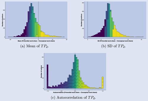
Figure 9. Primordial-conceptual word share difference across time. (a) Daily thinking process leaning across time. The figure plots the 25th and 75th (shaded area) quantiles and the average $T{P}_t$ for each year in the period 1890–2022 and (b) Monthly correlation of topics and primordial - conceptual word share difference across time and topics.

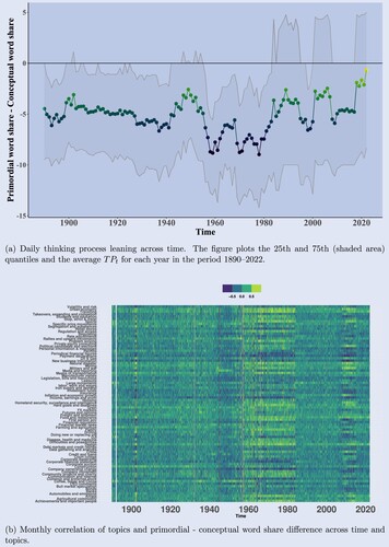
Figure 10. Narrative triggers of information sensitivity. The figure plots the ${\text{β}}_k^h$ coefficients of equation (8(8) $\begin{array}{rl}{\mathrm{\Delta }}_h{Y}_{i,t}& ={\alpha }_i^h+{\text{β}}_k^h\sum _{k=1}^{80}{A}_{k,t}+{\omega }_k^h\sum _{k=1}^{80}{F}_{i,t,k}+{\gamma }_k^h\sum _{k=1}^{80}{A}_{t,k}{F}_{i,t,k}\\ & +{\eta }^h{Z}_t+{\zeta }^h{X}_{i,t}+{ϵ}_t\mathrm{for}h=1,\dots ,30.\end{array}$(8) ) with 95% confidence intervals for topics with a positive and significant last period coefficients and at least 15 coefficients that are statistically significant at a 5% level between 1–30 day horizons. Statistical significance is calculated with standard errors clustered at the day and company level.

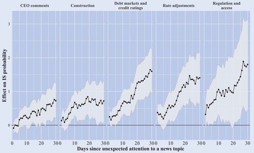
Figure 11. Individual company attention and narrative triggers of information sensitivity. The figure plots the ${\text{β}}_k^h$ and the ${\gamma }_k^h$ coefficients of equation (8(8) $\begin{array}{rl}{\mathrm{\Delta }}_h{Y}_{i,t}& ={\alpha }_i^h+{\text{β}}_k^h\sum _{k=1}^{80}{A}_{k,t}+{\omega }_k^h\sum _{k=1}^{80}{F}_{i,t,k}+{\gamma }_k^h\sum _{k=1}^{80}{A}_{t,k}{F}_{i,t,k}\\ & +{\eta }^h{Z}_t+{\zeta }^h{X}_{i,t}+{ϵ}_t\mathrm{for}h=1,\dots ,30.\end{array}$(8) ) with 95% confidence intervals for topics with a positive and significant last period coefficients and at least 15 coefficients that are statistically significant at a 5% level between 1–30 day horizons. Statistical significance is calculated with standard errors clustered at the day and company level.

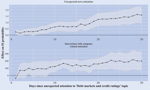
Figure 12. Narrative triggers of information sensitivity and different economic states. The figure plots the ${\text{β}}_k^h$ coefficients of equation (8(8) $\begin{array}{rl}{\mathrm{\Delta }}_h{Y}_{i,t}& ={\alpha }_i^h+{\text{β}}_k^h\sum _{k=1}^{80}{A}_{k,t}+{\omega }_k^h\sum _{k=1}^{80}{F}_{i,t,k}+{\gamma }_k^h\sum _{k=1}^{80}{A}_{t,k}{F}_{i,t,k}\\ & +{\eta }^h{Z}_t+{\zeta }^h{X}_{i,t}+{ϵ}_t\mathrm{for}h=1,\dots ,30.\end{array}$(8) ) with 95% confidence intervals for topics with positive and significant last period coefficient and at least 15 coefficients in total that are positive and statistically significant at a 5% level between 1–30 day horizons in at least one state. Statistical significance is calculated with standard errors clustered at the day and company level. The strong (red) coefficients refer to coefficients in the economically strong state and the weak (blue) refer to coefficients in the economically weak state.

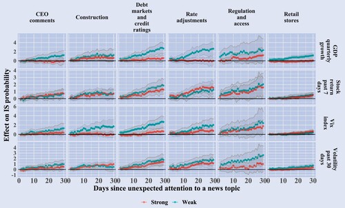
Figure 13. Narrative triggers of information sensitivity and different economic states. The figure plots the ${\text{β}}_k^h$ coefficients of equation (8(8) $\begin{array}{rl}{\mathrm{\Delta }}_h{Y}_{i,t}& ={\alpha }_i^h+{\text{β}}_k^h\sum _{k=1}^{80}{A}_{k,t}+{\omega }_k^h\sum _{k=1}^{80}{F}_{i,t,k}+{\gamma }_k^h\sum _{k=1}^{80}{A}_{t,k}{F}_{i,t,k}\\ & +{\eta }^h{Z}_t+{\zeta }^h{X}_{i,t}+{ϵ}_t\mathrm{for}h=1,\dots ,30.\end{array}$(8) ) with 95% confidence intervals for selected group of topics for which the coefficients are not statistically significant at a 5% level between 1–30 day horizons. Statistical significance is calculated with standard errors clustered at the day and company level. The strong (red) coefficients refer to coefficients in the economically strong state and the weak (blue) refer to coefficients in the economically weak state.

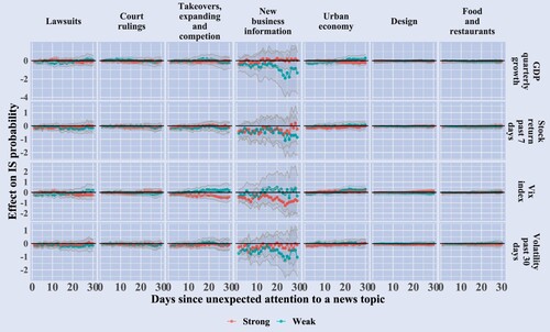
Figure 14. Journalists' thinking process-related language and narrative triggers of information sensitivity. The figure plots the ${\text{β}}_{l,k}^h$ coefficients of equation (11(11) $\begin{array}{rl}{\mathrm{\Delta }}_h{Y}_{i,t}& ={\alpha }_i^h+{\text{β}}_k^h\sum _{k=1}^{80}{A}_{k,t}+{\text{β}}_{l,k}^h\sum _{k=1}^{80}{L}_t{A}_{k,t}+{\omega }_k^h\sum _{k=1}^{80}{F}_{i,t,k}\\ & +{\omega }_{l,k}^h\sum _{k=1}^{80}{L}_t{F}_{i,t,k}+{\gamma }_k^h\sum _{k=1}^{80}{A}_{t,k}{F}_{i,t,k}\\ & +{\gamma }_{l,k}^h\sum _{k=1}^{80}{L}_t{A}_{t,k}{F}_{i,t,k}+{\eta }^h{Z}_t+{\zeta }^h{X}_{i,t}\\ & +{ϵ}_t\mathrm{for}h=1,\dots ,30.\end{array}$(11) ) with 95% confidence intervals for statistically significant trigger topics where the last period, and at least 15 ${\text{β}}_{l,k}^h$ coefficients overall, are statistically significant at a 5% level between 1–30 day horizons. Statistical significance is computed with standard errors clustered at the day and company level.

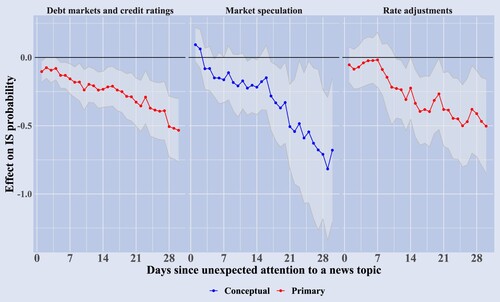
Table A1. Topic labels and the predictability of the attention to topics 1–40.

Topic	Common words	MAE	Positive surprises %
Rate adjustments	Rate fix reduction percentage reduce adjust effect	0.186	60
Construction	Line construction facility terminal bridge construct connect	0.155	65
Hard goals and deadlines	Goal tough role tie deadline match hurdle	0.279	63
Freight and shipment	Import loading shipment coin gold bulk freight	0.114	76
Bonds	Certificate reorganization proceed obligation date bondholder coupon	0.186	58
Segregation and substances	Give pacific reading tobacco observe telegraph carbide	0.05	66
FX markets	Sterling mark check lira call guilde belgian	0.134	66
Regulation and access	Free regulation commerce incentive barrier postal unlimited	0.065	71
Rallies and upward movements	Trend rubber narrow curb rally dealing early	0.168	53
Urban economy	Resident town city casino rural shelter gambling	0.28	65
Housing	Estate building property owner rent office tenant	0.295	57
Legislation, bills and resolutions	Tax adopt legislation bill resolution eliminate impose	0.312	63
Inflation and economic growth	Economy economic spending inflation economist boost euro	0.897	58
Credit and loans	Credit card loan lender borrower paper commercial	0.312	55
Difficulties and possibilities	Country difficulty circle possibility doubt circumstance prosperity	0.142	65
Corporate financial statement	Expect revenue cost gross result margin operating	0.301	51
Natural disaster	Fire disaster waste escape blame earthquake explosion	0.319	62
Oil & Gas	Natural gasoline gas energy pipeline gallon fuel	0.34	61
Financial market news	Small telephone clearing demand premium flat keen	0.061	58
Family	Family learn church mother son child lesson	0.357	71
Common and preferred stock	Stockholder stock common purchase prefer capitalization share	0.24	53
Court rulings	Decision ruling appeal answer legal question court	0.405	62
Permits	Permit road application railway grant permission necessary	0.104	68
Financial regulation	Financial regulator regulatory unit crisis collapse oversee	0.228	58
Stop, strict & insist	Rule mail implement stop strict insist editorial	0.097	65
Students and education	Student university op graduate education job academic	0.443	69
Doing new or replacing old	Take new step advantage symbol change helm	0.135	57
Lawsuits	bankruptcy Protection lawsuit filing file sue seek	0.291	59
Periodical financial figures	Increase figure year less compare period decrease	0.2	57
Disease, health and medicine	Drug study patient doctor disease cancer researcher	0.73	55
Sports	Team game player league pitch baseball football	0.73	59
Community projects and charity	Co complex community project found founder charity	0.147	66
Agricultural commodity	Wool textile sight cotton worth fertilizer south	0.069	63
Retail stores	Store retailer retail brand consumer shopper competition	0.353	59
Large movements	Rise drop jump climb lift surge index	0.442	51
Iron supply and demand	Iron pig inquiry concession basic foundry trade	0.07	60
Crime	Criminal prosecutor probe crime arrest jury guilty	0.8	60
Achievements and important people	Event honor revolution fortune moral self forget	0.334	66
Market speculation	Advance buying bull tendency selling speculative considerable	0.144	57
Labor, work and wages	Worker labor wage employ strike employment salary	0.178	67

Notes: The table presents the most common words for each topic calculated by the term frequency measure that takes into account the exclusivity and the frequency of each word. MAE refers to the Mean Absolute Error from the rolling window out-of-sample forecast made by the machine learning algorithm with information from past topic frequencies. The last column presents the percentage share of positive surprises (prediction errors) from all surprises.

Table A2. Topic labels and the predictability of the attention to topics 41–80.

Topic	Common words	MAE	Positive surprises %
Media and reporting	Press receive detail appear available comparison arrive	0.159	53
Specific price movements	Price level low high ounce pound depressed	0.24	57
Volatility and risk	Analyst emerge volatility investor risky cap volatile	0.418	51
Automobiles and emissions	Auto vehicle emission battery truck solar carbon	0.45	62
Design	Designer wall bedroom shirt clothe window style	1.339	54
Means of transportation	Air train airline flight plane driver passenger	0.436	61
Personal information & messages	Information personal employee message foundation define social	0.198	66
Artists	Music artist theater theatre novel song dance	1.215	65
Farming and agriculture	Farmer condition agricultural farm progress normal excellent	0.179	70
First person pov	Go get way many want one come	0.344	57
Regulating	Require law comply regulate state prohibit commissioner	0.207	66
Data gathering and analysis	Accord number datum analysis collect person release	0.155	62
Income, earnings and profit	Depreciation equal income equivalent net earn taxis	0.221	50
Communication and internet	Network ad search web advertising phone mobile	0.517	56
Corporate leadership	President board vice member chairman secretary senior	0.343	61
Private equity consulting	Partner strategy brokerage equity client top consulting	0.241	52
Debt markets and credit ratings	Term raise debt rating finance swap downgrade	0.216	58
Investment funds	Invest mutual investment fund pension manage asset	0.538	55
Coffee, Sugar and Cocoa	Point close bag unchanged sugar steady closing	0.099	55
Corporate auction	Bid municipal corporate auction offer bidder syndicate	0.219	58
Company ownership change	Plan acquire merger announce company ownership shareholder	0.288	55
Military and war	Military army troop regime rebel militant civilian	0.746	67
Travelling	Visit cross trip vacation rich bind obstacle	0.159	62
Payment declarations	Pay declare distribution payment declaration annual sum	0.146	60
Grain	Bushel wheat northwest grain winnipeg argentine visible	0.05	62
New business information	Business make understand important fact present enterprise	0.163	60
Political candidates and elections	Party election campaign presidential candidate voter debate	0.95	63
Takeovers, expanding and competition	Stake takeover venture expand customer competitor compete	0.311	51
Insurance	Care insurance familiar people insurer coverage matter	0.341	69
Drilling	Drill sand produce drilling spill gravity deep	0.14	64
Banks	Banking bank banker saving institution currency central	0.281	55
Food and restaurants	Food restaurant ice eat drink cup dog	0.886	56
Mining	Coal copper mine ore lake shipping vessel	0.134	66
Homeland security, surveillance and intelligence	Agency official administration citizen protect intelligence ministry	0.351	67
Dow Jones Industrial Average	Current value industrial average appreciation list secondary	0.103	69
Futures and options	Contract near commodity deliver dealer derivative position	0.1	53
Problem solving	Solution problem tool process experiment try rely	0.22	60
CEO comments	Chief executive address interview conference say comment	0.303	61
Company movement	Begin put set recent several bring similar	0.03	59
Manufacturer metals	Material steel manufacturer capacity manufacture scrap tin	0.108	59

Notes: The table presents the most common words for each topic calculated by the term frequency measure that takes into account the exclusivity and the frequency of each word. MAE refers to the Mean Absolute Error from the rolling window out-of-sample forecast made by the machine learning algorithm with information from past topic frequencies. The last column presents the percentage share of positive surprises (prediction errors) from all surprises.

Data availability statement

The paper uses text data from ProQuest historical newspapers. The actual text data is proprietary and it cannot be shared publicly. The data collection procedure is documented in detail in the paper. The website for ProQuest Historical newspapers is https://about.proquest.com/en/products-services/pq-hist-news/https://about.proquest.com/en/products-services/pq-hist-news/. One needs to have a payed subscription to the database to get access to the actual text data. In addition, the CDS spread data is proprietary and it cannot be shared publicly. It has been collected from Refinitiv Datastream and one needs to have a payed subscription to the database to get access to the CDS data.