Cross-section without factors: a string model for expected returns

Figures & data

Table 1. This table provides a heuristic construction of the expected return required to hold any asset i. The second column indicates how asset-i is exposed to fluctuations of any asset j. The second column is the unit risk premium required to bear a given exposure to any asset j, ${\varphi }_j\equiv \varphi ({\mathbf{y}}_t,j)$. The correlation premium, $\mathcal{C}$, is the average of the exposures weighted by the unit risk premia.

	Exposure to asset-j	Compensation	Premium
j = 1	$\sigma ({\mathbf{y}}_t,i)\rho ({\mathbf{y}}_t,i,1)$	${\varphi }_1$	$\sigma ({\mathbf{y}}_t,i)\rho ({\mathbf{y}}_t,i,1){\varphi }_1$
···	···	···	···
j = J	$\sigma ({\mathbf{y}}_t,i)\rho ({\mathbf{y}}_t,i,J)$	${\varphi }_J$	$\sigma ({\mathbf{y}}_t,i)\rho ({\mathbf{y}}_t,i,J){\varphi }_J$
			$\mathcal{C}=\sigma ({\mathbf{y}}_t,i)\frac{1}{J}\sum _{j=1}^J\rho ({\mathbf{y}}_t,i,j){\varphi }_j$

Figure 1. This picture depicts the average correlation exposure for 25 Size and Book-to-Market sorted portfolios, defined as ${\rho }_t^{\mathrm{\$}}=\frac{1}{n}\sum _{i=1}^n\sum _{j=1}^n{\rho }_t^{\mathrm{\$}}(i,j)$, where ${\rho }_t^{\mathrm{\$}}(i,j)$ is the realized correlation between portfolios j and i, obtained through a rolling window equal to 22 days.

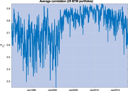
Figure 2. This figure plots three-month moving averages of the estimates of $y_t$, the state variable driving market correlations (red line), along with the University of Michigan Consumer Sentiment (UMCSENT) index (blue line). Both variables are de-meaned and standardized by their own standard deviations. The yellow shaded areas cover recession episodes as determined by the National Bureau of Economic Research.

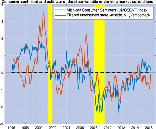
Figure 3. This picture plots the realized premium for correlation risk for S&P 500 stocks, defined as the difference between (i) risk-adjusted expectations of one-month average correlations, and implied by option prices, and (ii) realized correlations, calculated throughout a one-month window.

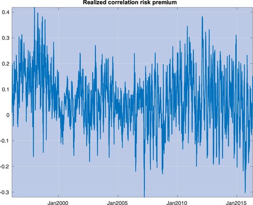
Figure 4. This picture plots the one-month premium for correlation risk $\mathcal{P}(y_t;\vartheta )$ in equation (21(21) $\begin{array}{rl}& \mathcal{P}(y_t;\vartheta )\\ & =\frac{{\varrho }_1}{T-t}{\int }_t^T(u(y_t,\tau -t;\theta ,\nu )-u(y_t,\tau -t;\theta ,0))\mathrm{d}\tau ,\end{array}$(21) ) against the state variable $y_t$ (left panel) and the average correlation predicted by the model, $\rho (y_t;\varrho )$ in equation (18(18) $\rho (y_t;\varrho )={\iint }_{i,j\in {[0,1]}^2}\rho (y_t;i,j)\mathrm{d}i\mathrm{d}j={\varrho }_0+{\varrho }_1{e}^{-y_t},$(18) ) (right panel). Parameter values are set equal to their estimates obtained in Section 4 (see table 2). The red line is the unconditional expected value of the premium for correlation risk predicted by the model, i.e. $E\left(\mathcal{P}\right(y_t;\vartheta \left)\right)$ in equation (26(26) $E\left(\mathcal{P}(y_t;\vartheta )\right)=\frac{{\varrho }_1}{T-t}{\int }_0^{T-t}(\overline{u}(x;\theta ,\nu )-\overline{u}(x;\theta ,0))\mathrm{d}x,$(26) ).

Table 2. GMM estimates of ${\hat{\zeta }}_N$ in (27(27) ${\hat{\zeta }}_N=\arg \underset{\zeta }{min}{h}_N\left(\zeta {)}^{⊺}{W}_N{h}_N\right(\zeta ),$(27) ) and t-stats.

	Estimate	t-stat
${\varrho }_0$	0.1779	7.23
$\ln {\varrho }_1$	−0.7460	−3.71
κ	3.8753	3.81
m	2.2423	2.71
η	4.1688	2.87
ν	3.3518	15.97

Figure 5. The top panel depicts estimates of the pro-cyclical state variable, $y_t$, obtained by matching the model predictions on realized correlations and the premium for correlation risk, as in equation (28(28) ${\hat{y}}_t=\arg \underset{y_t}{min}(\frac{({\rho }_t^{\mathrm{\$}}-\rho (y_t;{\hat{\varrho }}_{{}_N}){)}^2}{\mathrm{var}\left({\rho }_t^{\mathrm{\$}}\right)}+\frac{({\mathcal{P}}_t^{\mathrm{\$}}-\overline{\mathcal{P}}({\hat{\vartheta }}_N){)}^2}{\mathrm{var}\left({\mathcal{P}}_t^{\mathrm{\$}}\right)}),$(28) ). The bottom panel depicts the average correlation in the data (solid, blue line) and the average correlation predicted by the model (dashed, red line). The numbered circles identify events described in table 3.

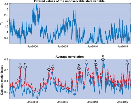
Table 3. This table provides descriptions of the major events leading to the spikes in correlation depicted in Figure 5.

Event	Date	Description
1	Nov 1997	Asian crisis corrections
2	Sep 1998	Russian financial crisis
3	Sep 2002	Bear market corrections
4	Mar 2003	Iraq War
5	Sep 2007	Subprime crisis
6	Sep 2008	Lehman Brothers bankruptcy
7	Jun 2010	European debt crisis I: Greece bailout
8	Aug 2011	European debt crisis II: spreading
9	Aug 2015	Chinese market corrections

Table 4. This table provides parameter estimates of $\overline{\varphi }$ in the constant string premium Model I, $\varphi (y_t,j)=\overline{\varphi }$ (with t-stats below), and the pricing performance expressed as the average pricing error (α is annualized) across a given set of portfolios, and the fit of the model (adjusted-$R^2$, ${\overline{R}}^2$) from this regression.

	$\overline{\varphi }$	α	${\overline{R}}^2$
5×5 ME-BTM	0.315	0.078	$-0.020$
	0.540	1.881	–
5×5 ME-INV	0.434	0.073	0.016
	1.242	2.893	–
5×5 ME-MOM	0.136	0.099	$-0.035$
	0.552	4.711	–
5×5 ME-REV	0.878	0.033	0.196
	3.070	1.442	–
5×5 ME-OP	−0.002	0.101	$-0.043$
	−0.004	2.978	–
5×5 ME-BTM Global	−0.307	0.103	$-0.033$
	−0.448	2.267	–

Table 5. This table provides parameter estimates of ${\varphi }_0$ and ${\varphi }_1$ in the cross-sectional variation premium Model II, $\varphi (y_t,j)={\varphi }_0{\varrho }_0\left(j\right)+{\varphi }_1{\varrho }_1\left(j\right)$ (with t-stats below) and the pricing performance expressed as the average pricing error (α is annualized) across a given set of portfolios, and the fit of the model (adjusted-$R^2$, ${\overline{R}}^2$) from this regression.

	${\varphi }_0$	${\varphi }_1$	α	${\overline{R}}^2$
5×5 ME-BTM	26.377	−15.188	0.181	0.235
	2.646	−2.248	2.618	–
5×5 ME-INV	51.991	−27.727	0.195	0.373
	3.547	−3.345	4.344	–
5×5 ME-MOM	34.776	−17.782	0.145	0.736
	11.921	−11.604	12.728	–
5×5 ME-REV	34.718	−16.770	0.102	0.502
	4.434	−4.156	5.608	–
5×5 ME-OP	86.275	−45.169	0.233	0.795
	10.309	−10.121	11.117	–
5×5 ME-BTM Global	70.577	−38.144	0.219	0.746
	7.191	−7.480	9.251	–

Table 6. This table provides parameter estimates of ${\varphi }_{v0}$, ${\varphi }_{v1}$ and ${\varphi }_{v2}$ in the time and cross-sectional variation premium Model III, $\varphi (y_t,j)={\varphi }_{v0}{\varrho }_0\left(j\right)+({\varphi }_{v1}+{\varphi }_{v2}{e}^{-y_t}){\varrho }_1\left(j\right)$ (with t-stats below), and the pricing performance expressed as the average pricing error (α is annualized) across a given set of portfolios, and the fit of the model (adjusted-$R^2$, ${\overline{R}}^2$) from this regression.

	${\varphi }_{v0}$	${\varphi }_{v1}$	${\varphi }_{v2}$	α	${\overline{R}}^2$
5×5 ME-BTM	−1.492	12.596	−30.290	0.132	0.330
	−0.076	0.696	−1.654	2.042	–
5×5 ME-INV	75.497	−49.833	24.470	0.212	0.417
	3.676	−2.865	1.276	6.003	–
5×5 ME-MOM	37.126	−20.059	2.667	0.145	0.737
	3.543	−2.107	0.255	12.471	–
5×5 ME-REV	27.276	−9.775	−7.894	0.099	0.507
	1.652	−0.673	−0.490	4.836	–
5×5 ME-OP	138.671	−92.983	53.900	0.238	0.891
	11.149	−9.358	5.584	15.532	–
5×5 ME-BTM Global	42.508	−14.140	−25.249	0.218	0.784
	2.669	−1.163	−2.158	9.264	–

Table 7. This table provides adjusted-$R^2$ from linear factor model regressions across the portfolios analzyed in tables 4 through 6. The four columns provide the adjusted-$R^2$ for the CAPM, the 3-F model (market, value, and size), the 4-F model (market, value, size, and momentum), and the 5-F model (market, size, value, profitability, and investment factors).

	CAPM	3-F	4-F	5-F
5×5 ME-BTM	0.168	−0.040	0.186	0.299
5×5 ME-INV	0.130	0.442	0.487	0.536
5×5 ME-MOM	0.348	−0.019	0.697	0.369
5×5 ME-REV	0.216	0.145	0.225	0.195
5×5 ME-OP	0.482	0.105	0.618	0.733
5×5 ME-BTM Global	−0.011	0.117	0.202	0.251

Figure 6. This picture depicts average excess returns and Model III predictions on the unconditional expected excess returns (the unconditional correlation premium of Proposition 3.2), for 5×5 ME-BTM, 5×5 ME-INV, 5×5 ME-MOM, 5×5 ME-REV, 5×5 ME-OP, and 5×5 ME-BTM Global portfolios.

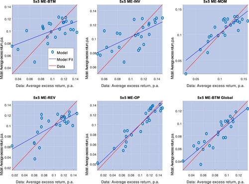
Figure 7. This picture depicts average excess returns and the unit risk premia for each portfolio, with the latter estimated from Model III. The estimates are performed for 5×5 ME-BTM, 5×5 ME-INV, 5×5 ME-MOM, 5×5 ME-REV, 5×5 ME-OP, and 5×5 ME-BTM Global portfolios.

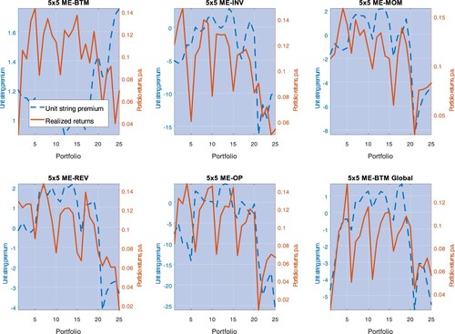
Figure 8. This picture depicts average excess returns and the sensitivity of the conditional sensitivity, ${\varrho }_1\left(j\right)$, for each portfolio, with the latter estimated from Model III. The estimates are performed for 5×5 ME-BTM, 5×5 ME-INV, 5×5 ME-MOM, 5×5 ME-REV, 5×5 ME-OP, and 5×5 ME-BTM Global portfolios.

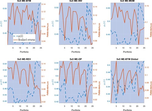
Figure 9. This picture depicts quarterly realized returns of portfolios sorted by size in the first decile (dashed, blue line) and the tenth decile (‘big size’) (dashed, blue line). The numbered circles identify the same events in figure 5 (see table 3) and are placed around the realization of big size portfolios returns.

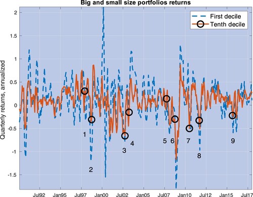
Figure 10. This picture depicts the relation between the conditional correlation premium predicted by Model III (equally weighted across all portfolios) and the state variable $y_t$ regarding 5×5 ME-BTM, 5×5 ME-INV, 5×5 ME-MOM, 5×5 ME-REV, 5×5 ME-OP, and 5×5 ME-BTM Global portfolios. The red, horizontal line is the unconditional premium for each of these portfolios.

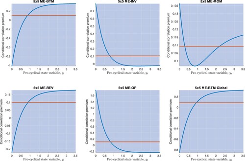
Figure 11. This picture depicts scatterplots of realized premium for correlation risk for S&P 500 stocks against one-month realized correlations. Blue and red dots identify pairs in the data and pairs predicted by the model, respectively.

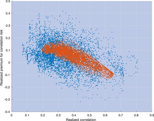
Figure 12. This picture depicts the unconditional premium for correlation risk calculated for horizons equal to 1, 3, 6, 9, and 12 months. The circles are data estimates, computed as described in the main text. The solid curve depicts model predictions, obtained while fixing parameter values at the GMM estimates in (27(27) ${\hat{\zeta }}_N=\arg \underset{\zeta }{min}{h}_N\left(\zeta {)}^{⊺}{W}_N{h}_N\right(\zeta ),$(27) ), which rely on one moment condition based on one-month unconditional premium.

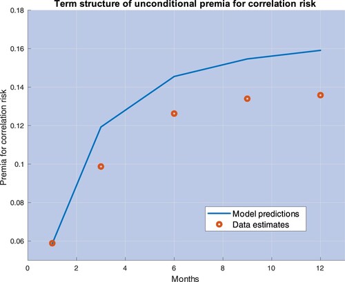
Table 8. This table provides estimates (with standard errors in parenthesis) and adjusted-$R^2$ for the coefficients a and b in the linear regression ${\rho }_Q=a+b{\rho }_P$, where ${\rho }_Q$ is the one-month expected correlation for S&P 500 stocks under the risk-neutral probability, Q, and ${\rho }_P$ is the one-month realized correlation.

	a	b	${\overline{R}}^2$
Data	(0.0034)	(0.0096)	46%
	0.1804	0.6337
Model	(0.0015)	(0.0038)	76%
	0.2508	0.4913

Table D1. This table provides parameter estimates of ${\varphi }_{v0}$, ${\varphi }_{v1}$ and ${\varphi }_{v2}$ in the time and cross-sectional variation premium Model III, $\varphi (y_t,j)={\varphi }_{v0}{\varrho }_0\left(j\right)+({\varphi }_{v1}+{\varphi }_{v2}{e}^{-y_t}){\varrho }_1\left(j\right)$ (with t-stats below), and the pricing performance expressed as the average pricing error (α is annualized) across a given set of portfolios, and the fit of the model (adjusted-$R^2$, ${\overline{R}}^2$) from this regression. The first column provides the number of stocks in each portfolio (J). The last line provides the average adjusted-$R^2$ across all portfolios for each model.

	J	${\varphi }_{v0}$	${\varphi }_{v1}$	${\varphi }_{v2}$	α	${\overline{R}}^2$
ENERGY	34	−34.458	19.024	−1.129	0.055	0.513
		−2.890	1.937	−0.113	1.612	–
MATERIALS	32	−76.475	37.816	−5.737	0.110	0.517
		−1.763	1.350	−0.274	4.712	–
INDUSTRIALS	76	132.112	−70.574	41.356	0.073	0.181
		1.700	−1.799	2.354	2.303	–
CONS. DISCRET.	79	51.391	−28.591	20.876	0.086	0.088
		0.969	−0.931	0.926	3.674	–
CONS. STAPLES	35	−98.597	24.520	35.578	0.294	0.523
		−1.229	0.462	0.775	4.318	–
HEALTH	48	−62.965	30.130	−1.497	0.003	0.401
		−0.747	0.610	−0.046	0.070	–
FINANCIALS	71	−30.543	13.839	−1.601	0.116	0.636
		−6.684	3.863	−0.308	7.081	–
TECHNOLOGY	51	49.876	−43.341	50.427	0.108	0.189
		2.253	−2.674	3.060	2.119	–
UTILITIES	28	−15.420	11.473	−13.129	0.179	0.374
		−1.055	0.823	−0.866	10.235	–
SP 100	107	−14.767	2.637	8.127	0.102	0.049
		−0.892	0.229	0.653	5.905	–
DOW JONES 30	37	48.786	-46.909	60.455	0.071	0.151
		1.761	−2.344	2.737	2.023	–
NASDAQ 100	109	−41.579	7.477	25.557	0.052	0.256
		−1.616	0.551	2.732	1.959	–
Average ${\overline{R}}^2$						0.429

Table D2. This table provides adjusted-$R^2$ from linear factor model regressions across the portfolios in Table A1. The first column provides the number of stocks in each portfolio (J). The second through the fourth provide adjusted-$R^2$ for the CAPM, the 3-F model (market, value, and size), the 4-F model (market, value, size, and momentum), and the 5-F model (market, size, value, profitability, and investment factors). The last line provides the average adjusted-$R^2$ across all portfolios for each model.

	J	CAPM	3-F	4-F	5-F
ENERGY	34	0.216	0.311	0.431	0.344
MATERIALS	32	0.092	0.214	0.306	0.347
INDUSTRIALS	76	0.079	0.157	0.449	0.350
CONS. DISCRET.	79	−0.001	0.210	0.345	0.266
CONS. STAPLES	35	−0.028	0.143	0.408	0.184
HEALTH	48	0.492	0.633	0.731	0.668
FINANCIALS	71	0.026	0.247	0.299	0.267
TECHNOLOGY	51	0.134	0.305	0.506	0.386
UTILITIES	28	0.677	0.650	0.748	0.750
SP 100	107	0.092	0.313	0.524	0.297
DOW JONES 30	37	−0.020	0.110	0.371	0.342
NASDAQ 100	109	0.074	0.130	0.346	0.224
Average ${\overline{R}}^2$	–	0.178	0.226	0.436	0.379

Data availability

The authors confirm that the data supporting the findings of this study are available within its supplementary materials (available upon request).