Figures & data
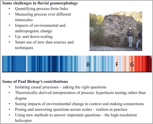
Figure 1. A sand-bed river in Victoria, Australia with floodplain and in-channel sediments influenced by post-European settlement erosion (see Portenga et al., Citation2016). I forget the precise location, but the image is memorable as the photograph was taken on the day when I first met Paul Bishop.
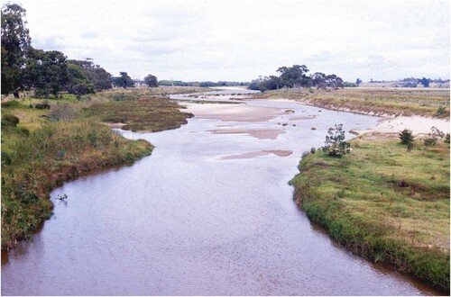
Figure 2. ‘Livestock standing in a small farm dam’ (start of original caption from Lloyd et al., Citation1998).
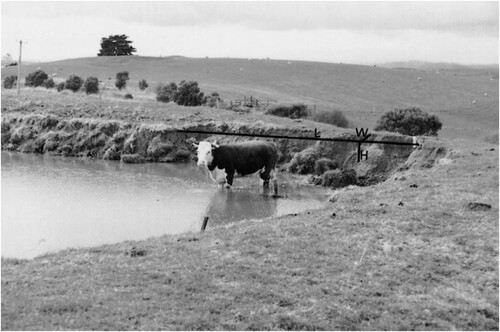
Figure 3. (a) Catchments of the Sierra Nevada, Spain. Catchments labelled N drain northwards from the range, and those labelled S drain south towards the Mediterranean Sea. (b) River slope (red/lighter line) determined from GTOPO30 Digital Elevation Model and catchment area, for the Picena River (catchment S6). Note abrupt increases in catchment area at tributary junctions. (c) Normalised long profiles for the north (red/lighter) and south (black/darker) draining rivers. Unpublished data from John Jansen.
Figure 4. Field data and model results from van der Beek and Bishop (Citation2003). (a) Long profiles of the present-day Lachlan River, Australia and fluvial terraces, showing locations of the 12.5 Ma Boorowa basalt and alluvial fill at the bedrock-alluvial transition. (b) Modern river profiles for the Lachlan River and three tributary creeks predicted by two incision models, each of which includes variable lithologies shown in the boxes below each profile. Grey shading shows the Adaminaby Group metamorphics and white is the Wyangala Granite. (c) Results of Monte Carlo sampling of the parameter space for one of the models tested by van der Beek and Bishop (Citation2003), the tools model. Plots show root mean square (RMS) of model misfit against four model parameters (mt, nt are exponents and normalised Kt is a constant in a transport-limited fluvial incision law, and Lf is a characteristic length scale for incision).
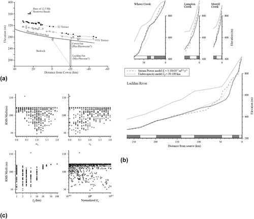
Figure 5. Relationships between sediment cover (Fe) and relative sediment supply (Qs/Qt, where Qs is sediment supply and Qt is the capacity sediment transport rate in the channel). A range of different forms of this relationship (colour coded and groups 1–6 in the legend) are found for combinations of the probabilities of entrainment of isolated grains (Pi) and cluster grains (Pc). Reproduced from Hodge and Hoey (Citation2012).
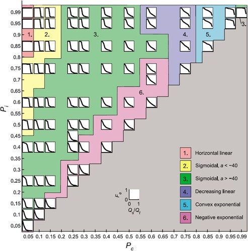
Figure 6. Bedrock river long profiles and knickpoints at different scales. (a)-(d) (Kim, Citation2004) show knickpoints on the River Etive, Scotland, including sculpted bedforms (b) and incision below a strath terrace (d). (e) is part of the long profile of the River Etive, showing exposed bedrock (grey shading), alluvial cover (thick grey line) and strath terraces (dashed line). 10Be exposure ages of the strath terrace are plotted on the right y-axis. From Jansen et al. (Citation2011). (f) SEM images (Kim, Citation2004) of bedrock plates from the River Etive following abrasion tests in a tumbling mill. Number on the upper image indicate different minerals (1 – feldspar; 2 – quartz). Arrows show impact marks from clasts in the tumbling mill. (g) Scaling of knickpoint retreat with catchment area for small streams along the east cost of Scotland (from Bishop et al., Citation2005).
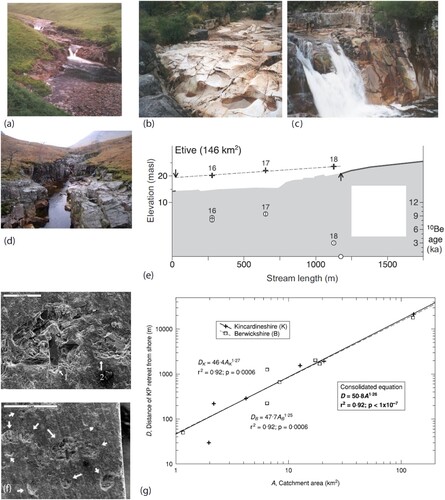
Figure 7. Erosion of the Sierra Nevada, Spain. (a) digital elevation model (Pérez-Peña et al., Citation2010) showing the overall E-W orientation of the mountain range, with the highest elevation terrain towards the western end. The Rio Torrente catchment is on the SW margin of the range. (b) View of the upper part of the Rio Torrente catchment, looking NE towards the peak of Cerro de Caballo (3005m). (c) Topographic map of the Rio Torrent catchment, showing in site and detrital 10Be erosion rates (Reinhardt et al., Citation2007a).
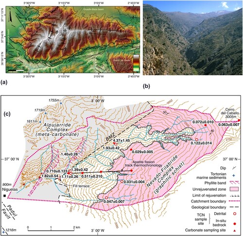
Figure 8. (a) View of the Rio Torrente catchment showing the contrast between rapid erosion below the knickpoints and slow erosion on the lower gradient upper catchment terrain (Reinhardt et al., Citation2007a). (b) Estimates of the number of erosion rate estimates (upper plot) required to generate standard error = 0.2 mean erosion rate as a function of erosion rate, spalling thickness (L) and detachment recurrence interval (T). Lower plot shows the relative standard error as a function of the number of samples (Reinhardt et al., Citation2007b). (c) Modelled measured (dashed lines) and mean (solid grey line) erosion rates for a 0.8m bedrock chip removed every 3000 years (Reinhardt et al., Citation2007b). (d) Relative 10Be concentrations for 8-16mm and 0.25-0.5mm size fractions in detrital sediment samples from the Rio Torrente (Reinhardt et al., Citation2007b).
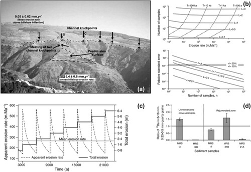
Figure 9. (a) Spatial distribution of mean slope in the upper Gaub River catchment (Namibia) (Codilean et al., Citation2008). (b) Normalised 21Ne concentration distributions for different assumptions regarding the timing of erosion (Codliean et al., Citation2009). (c) Cumulative frequency distribution from 32 measurements of 21Ne in individual clasts in Gaub River sediments. Inset shows simulated cumulative frequency distributions of 21Ne for two different assumptions of the dependence of erosion rate on catchment slope, and the hypsometry of the catchment (DEM) (Codliean et al., Citation2008).
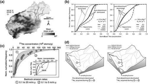
Figure 10. Summarising Paul’s career in context. Challenges are generalised (see Church, Citation2010). Photograph is of Paul (with hat) with Tim Dempster in the Sierra Nevada, Spain. Climate stripes from Hawkins (Citation2018) show the period 1850–2020. B – birth of Paul Bishop; F – date of his first paper as lead author (Bishop, Citation1980); G – Paul moves to University of Glasgow.