The influence of product instability on slow-binding inhibition

Figures & data

short-legendScheme 1

Figure 1 Progress curves of the species involved in Scheme 1 obtained by numerical solution of the set of differential equations that describes the kinetics of the enzyme system. The arbitrary values used for the initial concentrations and rate constants are: , ,

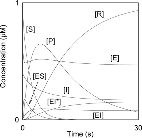
Figure 2 (a) Evaluation of t_inflex. A set of points with low values of d[P]/dt are chosen. These points are fitted using a polynomial of degree three. One root of the derivative of this polynomial is t_inflex. (b) Evaluation of t_∞. Data points at t < t_max, which are located near are chosen. These points are fitted using a polynomial of the degree two. One root of the equation is t_∞. (c) Evaluation of α₀. The first data points of d[P]/dt, i.e. data points at low t-values, are fitted using a polynomial of the degree two. The independent term of this polynomial is α₀.

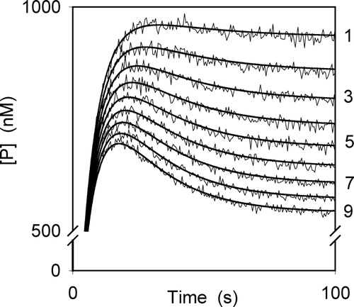
Figure 3 Progress curves simulated with added errors and calculated (continuous lines) using equation (9) corresponding to the proposed example. The values of the rate constants and initial concentrations used are: for the curves 1–9, respectively.

Figure 4 (a) Plot of [E]₀/(j[P]_∞) vs. 1/[S]₀ at constant [I]₀ according to equation (A29). (b) Plot of [E]₀/α₀ vs. 1/[S]₀ at constant [I]₀ according to equation (A31).

Figure 5 (a) Plot of ([S]₀[E]₀)/(j[P]_∞) vs. [I]₀ at constant [S]₀ according to equation (A29). (b) Plot of ([S]₀[E]₀)/α₀ vs. [I]₀ at constant [S]₀ according to equation (A31).