Identifying novel sphingosine kinase 1 inhibitors as therapeutics against breast cancer

Figures & data

Figure 1. The flowchart showing the ligand-based virtual screening of compounds.

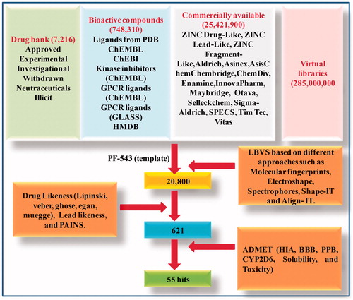
Table 1. Analysis of drug like properties of top 10 compounds and PF-543 on the basis of Lipinski’s RO5.

S. no.	Name of compounds	Molecular weight (g/mol)	H-bond donor	H-bond acceptor	A log P
1	ZINC06823429	341.45	1	4	3.39
2	ZINC95421501	346.49	1	3	2.14
3	ZINC95421070	344.47	1	4	2.99
4	ZINC95421502	346.49	1	3	2.14
5	ZINC04967864	342.44	1	5	2.98
6	ZINC97084836	329.46	1	3	3.44
7	ZINC72152243	348.50	1	4	1.36
8	ZINC84976927	348.51	0	5	2.09
9	19-Norandrostenedione	272.38	0	2	3.37
10	ZINC95975458	329.46	1	3	3.50
11	Standard drug PF-543	465.20	1	4	5.89

Table 2. ADMET calculation of top 10 compounds and PF-543.

S. no.	Name of compounds	HIA	BBB	PPB	CYP2D6	Solubility	Toxicity	A log P98	PSA2D
1	ZINC06823429	0	1	2	0	2	NC	3.58	52.63
2	ZINC95421501	0	2	0	0	3	NC	2.14	50.76
3	ZINC95421070	0	2	2	0	2	NC	2.99	50.76
4	ZINC95421502	0	2	0	0	3	NC	2.14	50.76
5	ZINC04967864	0	2	0	0	2	NC	3.17	63.89
6	ZINC97084836	0	1	2	0	2	NC	3.44	47.41
7	ZINC72152243	0	2	0	0	3	NC	1.36	44.82
8	ZINC84976927	0	2	0	0	3	NC	2.09	38.62
9	19-Norandrostenedione	0	1	0	0	2	NC	3.37	34.60
10	ZINC95975458	0	1	2	0	2	NC	3.50	47.41
11	Standard drug PF-543	0	1	2	0	2	NC	5.02	67.70

Table 3. Docking analysis of top 10 compounds and comparison with known drug.

S. no.	Name of compounds	Binding energy^a (kcal/mol)	Ki^b (μM)
1	ZINC06823429	–11.36	4.74
2	ZINC95421501	–11.29	5.31
3	ZINC95421070	–11.26	5.54
4	ZINC95421502	–11.16	6.59
5	ZINC04967864	–11.02	8.30
6	ZINC97084836	–10.71	14.21
7	ZINC72152243	–10.67	15.03
8	ZINC84976927	–10.65	15.62
9	19-Norandrostenedione	–10.47	21.05
10	ZINC95975458	–10.43	22.57
11	Standard drug PF-543	–9.90	55.04

^a Calculated free energy of binding (ΔG) in kcal/mol.

^b Calculated inhibition constant Ki from AutoDock Tools 4.2.

Figure 2. The binding mode of ZINC06823429 with the SphK1. (A) The overall structure of SphK1–ZINC06823429 complex showing protein in cartoon model and ligand in stick. (B) Interaction of ZINC06823429 to the SphK1 residues (stick). (C) 2D diagram of SphK1 interaction with the compound ZINC06823429. The active site residues of SphK1 interacting with ligand ZINC06823429 by four conventional H-bonds.

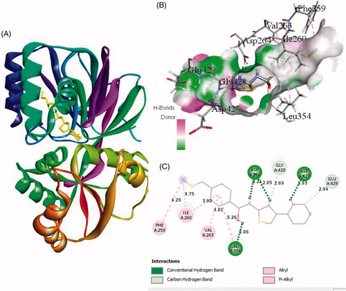
Figure 3. The binding mode of ZINC95421501 with the SphK1. (A) The overall structure of SphK1–ZINC95421501 complex showing protein in cartoon model and ligand in stick. (B) Interaction of ZINC95421501 to the SphK1 residues (stick). (C) 2D diagram of SphK1 interaction with the compound ZINC95421501. The active site residues of SphK1 interacting with ligand ZINC95421501 by two conventional H-bonds.

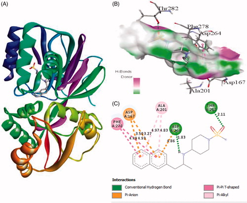
Figure 4. The binding mode of ZINC95421070 with the SphK1. (A) The overall structure of SphK1–ZINC95421070 complex showing protein in cartoon model and ligand in stick. (B) Interaction of ZINC95421070 to the SphK1 residues (stick). (C) 2D diagram of SphK1 interaction with the compound ZINC95421070. The active site residues of SphK1 interacting with ligand ZINC95421070 by three conventional H-bonds.

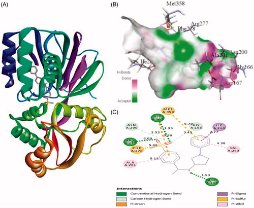
Figure 5. The binding mode of PF-543 with the SphK1. (A) The overall structure of SphK1–PF-543 complex showing protein in cartoon model and ligand in stick. (B) Interaction of PF-543 to the SphK1 residues (stick). (C) 2D diagram of SphK1 interaction with the compound PF-543. The active site residues of SphK1 interacting with ligand PF-543 by one conventional H-bonds.

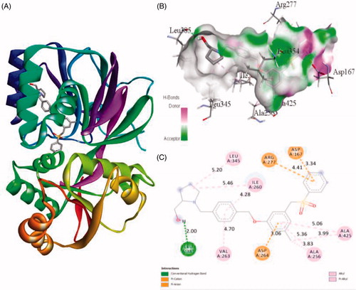
Table 4. Calculated parameters for all the systems obtained after 100 ns MD simulations.

Complexes	Average potential energy (kJ/mol)	Radius of gyration (nm)	Average RMSD (nm)	Average SASA (backbone, nm^2)	Free energy of solvation (kJ/mol/nm^2)	Volume (nm^3)	Density (g/l)
SphK1	–767,455	1.92	0.29	171.74	264.63	62.85	1015.11
SphK1–PF-543	–766,868	1.96	0.44	171.96	252.64	62.96	1013.30
SphK1–ZINC06823429	–766,795	1.93	0.34	168.93	255.25	63.07	1011.59
SphK1–ZINC95421070	–767,127	1.90	0.25	170.01	249.01	62.55	1019.99
SphK1–ZINC95421501	–766,972	1.92	0.27	171.82	268.47	62.94	1013.66

Figure 6. Dynamics of ligands binding to the SphK1. (A) RMSD plot as a function of time. Black, red, green, blue, and yellow colours represent values obtained for SphK1, SphK1–STD, SphK1–ZINC06823429, SphK1–ZINC95421070, and SphK1–ZINC95421501, respectively. (B) Comparison of orientations of PF-543 (red), ZINC06823429 (green), ZINC95421070 (blue), and ZINC95421501 (yellow) into the active pocket of SphK1. (C) Backbone atomic fluctuations (RMSF) plot for SphK1, SphK1–PF-543, SphK1–ZINC06823429, SphK1–ZINC95421070, and SphK1–ZINC95421501. (D) Time evolution of radius of gyration (R_g) values during 100,000 ps (100 ns) of MD simulation. The R_g plot for SphK1 is shown in black. Red, green, blue, and yellow colours represent R_g plot for SphK1–PF-543, SphK1–ZINC06823429, SphK1–ZINC95421070, and SphK1–ZINC95421501, respectively.

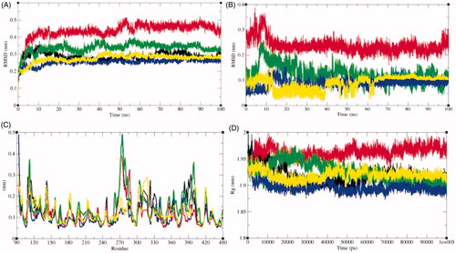
Figure 7. Solvent accessible surface area. (A) The solvent accessible surface area (SASA) as a function of time. Black, red, green, blue, and yellow colours represent values obtained for SphK1, SphK1–STD, SphK1–ZINC06823429, SphK1–ZINC95421070, and SphK1–ZINC95421501, respectively. The SASA plot was further resolved into hydrophobic and hydrophilic surface area for (B) SphK1, (C) SphK1–PF-543, (D) SphK1–ZINC06823429, (E) SphK1–ZINC95421070, and (F) SphK1–ZINC95421501, respectively.

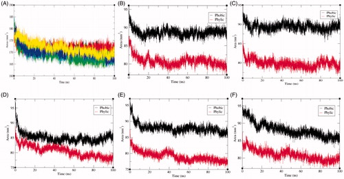
Figure 8. Free energy of solvation during SASA analysis. Free energy of solvation during SASA analysis was calculated for SphK1, SphK1–PF-543, SphK1–ZINC06823429, SphK1–ZINC95421070, and SphK1–ZINC95421501, respectively. Black, red, green, blue, and yellow colours represent the values obtained for SphK1, SphK1–PF-543, SphK1–ZINC06823429, SphK1–ZINC95421070, and SphK1–ZINC95421501, respectively.

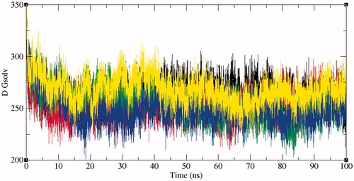
Figure 9. The average number of hydrogen bonds as a function of time. Red, green, blue, and yellow colours represent the number of hydrogen bonds for SphK1–PF-543, SphK1–ZINC06823429, SphK1–ZINC95421070, and SphK1–ZINC95421501, respectively.

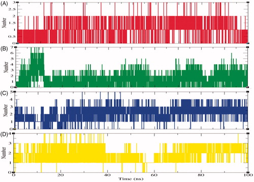
Figure 10. The secondary structure plot. The graphical representation indicating the structural elements present during 100 ns MD simulations in (A) SphK1, (B) SphK1–PF-543, (C) SphK1–ZINC06823429, (D) SphK1–ZINC95421070, and (E) SphK1–ZINC95421501, respectively.

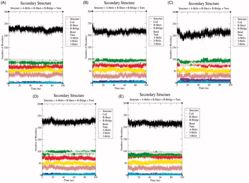
Figure 11. Position of ligands in the secondary structure framework. The secondary structure representation of SphK1 during 100 ns MD simulation in (A) SphK1, (B) SphK1–PF-543, (C) SphK1–ZINC06823429, (D) SphK1–ZINC95421070, and (E) SphK1–ZINC95421501, respectively.

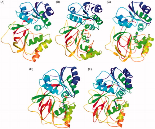
Table 5. Percentage of residues participated in average structure formation.

	Percentage of protein secondary structure (SS%)
Complexes	Structure^a	Coil	β-Sheet	β-Bridge	Bend	Turn	α-Helix	310-helix
SphK1	65%	19%	26%	1%	15%	10%	28%	1%
SphK1–PF-543	61%	21%	26%	2%	15%	9%	25%	1%
SphK1–ZINC06823429	59%	22%	26%	2%	15%	8%	23%	1%
SphK1–ZINC95421070	64%	20%	28%	1%	14%	9%	27%	1%
SphK1–ZINC95421501	62%	22%	25%	1%	15%	8%	27%	1%

^a Structure = α-helix + β-sheet + β-bridge + turn.

Figure 12. Principal component analysis (PCA). The PCA or essential dynamics (ED) calculated for SphK1, SphK1–PF-543, SphK1–ZINC06823429, SphK1–ZINC95421070, and SphK1–ZINC95421501, respectively. (A) The graph indicated the projection of eigenvectors in SphK1 (black), SphK1–PF-543 (red), SphK1–ZINC06823429 (green), SphK1–ZINC95421070 (blue), and SphK1–ZINC95421501 (yellow), respectively. (B) The Eigen root mean square fluctuations indicating the atomic fluctuations were also calculated for SphK1 (black), SphK1–PF-543 (red), SphK1–ZINC06823429 (green), SphK1–ZINC95421070 (blue), and SphK1–ZINC95421501 (yellow), respectively.

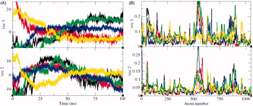
Figure 13. 2D projection of trajectories. The 2D projections of trajectories on eigenvectors showed different projections of SphK1 in case of (A) SphK1, (B) SphK1–PF-543, (C) SphK1–ZINC06823429, (D) SphK1–ZINC95421070, and (E) SphK1–ZINC95421501, respectively.

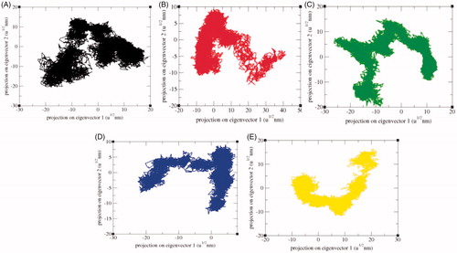
Table 6. Average binding energy calculation using g_mmpbsa package implemented in GROMACS for high-throughput MMPBSA calculation for protein–ligand complexes.

		Polar solvation energy (kJ/mol)			Vacuum MM energy (kJ/mol)			Average binding energy (kJ/mol)
S. no.	Complexes	Protein PB energy	LIG PB energy	Protein-LIG PB energy	Protein-LIG VdW energy	Protein-LIG Elec. energy	Protein-LIG total energy	van der Waals energy	Electrostatic energy	Binding energy
1	SphK1–PF-543	–9300	–272	–9135	–260	–430	–690	–259	–430	–276
2	SphK1–ZINC06823429	–9525	–775	–9051	–137	–1474	–1611	–138	–1474	–380
3	SphK1–ZINC95421070	–9085	–272	–9260	–40	–144	–155	–40	–115	–61
4	SphK1–ZINC95421501	–9151	–273	–8931	–219	–449	–668	–219	–449	–194