Models of enzyme inhibition and apparent dissociation constants from kinetic analysis to study the differential inhibition of aldose reductase

Figures & data

Figure 1. The secondary plot of apparent kinetic parameters ratio ^appK_M/^appk_cat versus [I] for the EGCG inhibition on HNE reduction. The dotted line refers to linear regression analysis fixing the intercept with the y-axis at the ^appK_M/^appk_cat control value. Each value represents the ^appK_M/^appk_cat ratio evaluated at the indicated EGCG concentrations. Data were obtained through non-linear regression analysis of v_o vs [S] measurements using the Michaelis Menten equation. Bars (when not visible are within the symbols size) represent the standard error of the measurements.

Figure 2. Inhibition models of an enzyme (E): a general model of inhibition (Panel A) and an alternative model of inhibition following “the classical approach” (Panel B). (S): substrate; (I): inhibitor; (ES): enzyme-substrate complex; (EI): enzyme-inhibitor complex; (EIS): enzyme-inhibitor-substrate ternary complex; k₊₁, k₋₁, k₊₂, k₊₃, k₋₃, k₊₄ refer to kinetic constants; K_i and K’_i refer to EI and EIS dissociation constants, respectively. See text for details.

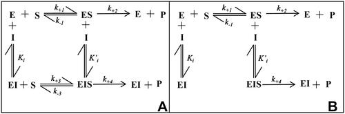
Figure 3. Incomplete uncompetitive inhibition. (Panel A) represents the dependence of ^appk_cat on the increase of [I] according to Equation (2)(2) $${}^{\mathit{app}}{k}_{\mathit{cat}}=\frac{{K_i^{\mathrm{*}}k}_{+2}+k_{+4}\left[I\right]}{K_i^{\mathrm{*}}+\left[I\right]}\mathrm{ }$$(2) ; (Panel B) represents the dependence of ^appk_M on the increase of [I] according to Equation (3)(3) $${}^{\mathit{app}}{K}_M=\frac{K_i^{\mathrm{*}}{K}_M+\frac{k_{+4}}{k_{+1}}\left[I\right]}{K_i^{\mathrm{*}}+\left[I\right]}$$(3) ; (Panel C) represents the dependence of ^appK_M/^appk_cat on the increase of [I] according to Equation (4)(4) $$\frac{{}^{\mathit{app}}{K}_M}{{}^{\mathit{app}}{k}_{\mathit{cat}}}=\frac{K_i^{\mathrm{*}}{K}_M+\frac{k_{+4}}{k_{+1}}\left[I\right]}{{K_i^{\mathrm{*}}k}_{+2}+k_{+4}\left[I\right]}$$(4) .

Figure 4. Predicted effect of the inhibitor concentration on the apparent kinetic parameters. The dependence of 1/^appk_cat (Panel A) and ^appK_M/^appk_cat (Panel B) on the inhibitor concentration for different incomplete uncompetitive inhibition situations is reported, according to Equations (2(2) $${}^{\mathit{app}}{k}_{\mathit{cat}}=\frac{{K_i^{\mathrm{*}}k}_{+2}+k_{+4}\left[I\right]}{K_i^{\mathrm{*}}+\left[I\right]}\mathrm{ }$$(2) and 4)(4) $$\frac{{}^{\mathit{app}}{K}_M}{{}^{\mathit{app}}{k}_{\mathit{cat}}}=\frac{K_i^{\mathrm{*}}{K}_M+\frac{k_{+4}}{k_{+1}}\left[I\right]}{{K_i^{\mathrm{*}}k}_{+2}+k_{+4}\left[I\right]}$$(4) , respectively. The following arbitrary values were fixed: k₊₂ = 1, k₊₁ = 100, K_M = 0.5 and $K_i^{\mathrm{*}}$ = 0.001. Curves 1–6 refer to k₊₄ values of zero (complete inhibition), 0.02, 0.05, 0.1, 0.15 and 0.2, respectively.

Figure 5. Predicted effect of the inhibitor concentration on the apparent kinetic parameters. The dependence of 1/^appk_cat (Panels A and D), ^appK_M (Panels B and E) and ^appK_M/^appk_cat (Panels C and F) on the inhibitor concentration for different incomplete mixed inhibition situations is reported, according to Equations (6–8), respectively. The following arbitrary values were fixed: k₊₂ = 1, k₊₁ = 100, K_M = 0.5. Curves 1–6 refer to k₊₄ values of zero (complete inhibition), 0.02, 0.05, 0.1, 0.15 and 0.2, respectively. (Panels A–C) refer to $K_i^{\mathrm{*}}$ and K_i values of 0.001 and 0.01, respectively. (Panels D–F) refer to $K_i^{\mathrm{*}}$ and K_i values of 0.01 and 0.001 respectively. In (Panels B and E), curves 1–6 are essentially superimposable. Having imposed a reasonable rather low value of k₊₂/k₊₁ (0.01), k₊₄/k₊₁ will be negligible making the curves of ^appK_M versus [I] at different k₊₄ are essentially superimposable.

Figure 6. Inhibition model of an enzyme (E) following “the non-classical approach”. (S): substrate; (I): inhibitor; (ES): enzyme-substrate complex; (EI): enzyme-inhibitor complex; (EIS): ternary enzyme-inhibitor-substrate complex; k₊₁, k₋₁, k₊₂, k₊₃, k₋₃, k₊₄ are kinetic constants; K_i is the EI complex dissociation constant. See text for details.

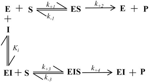
Figure 7. Non-classical approach for complete inhibition. (Panel A) represents the dependence of ^appK_M on the increase of [I] according to Equation (10)(10) $${}^{\mathit{app}}{K}_M=\frac{k_M\left(1+\frac{\left[I\right]}{K_i}\right)}{1+\frac{\left[I\right]k_M}{K_i{K}_M^{\mathrm{\prime }}}}\mathrm{ }$$(10) ; (Panel B) represents the dependence of 1/^appk_cat on the increase of [I] according to Equation (11)(11) $${}^{\mathit{app}}{k}_{\mathit{cat}}=\frac{{K_i{K}_M^{\mathrm{\prime }}k}_{+2}}{K_i{K}_M^{\mathrm{\prime }}+k_M\left[I\right]}$$(11) ; Panel C represents the dependence of ^appK_M/^appk_cat on the increase of [I] according to Equation (12)(12) $$\frac{{}^{\mathit{app}}{K}_M}{{}^{\mathit{app}}{k}_{\mathit{cat}}}=\frac{K_M}{k_{+2}}+\frac{K_M}{K_i{k}_{+2}}\left[I\right]\mathrm{ }$$(12) .

Figure 8. Non-classical approach for incomplete inhibition. (Panel A) represents the dependence of ^appK_M on the increase of [I] according to Equation (14)(14) $${}^{\mathit{app}}{K}_M=\frac{{K_{i}K}_M{K}_M^{\mathrm{\prime }}+K_M{K}_M^{\mathrm{\prime }}\left[I\right]}{{K_M^{\mathrm{\prime }}{K}_i+K}_M\left[I\right]}$$(14) ; (Panel B) represents the dependence of 1/^appk_cat on the increase of [I] according to Equation (15)(15) $${{}^{\mathit{app}}k}_{\mathit{cat}}=\mathrm{ }\frac{k_{+2}{K}_M^{\mathrm{\prime }}{K}_i+k_{+4}{K}_M\left[I\right]}{K_M^{\mathrm{\prime }}{K}_i{+\mathrm{ }K}_M\left[I\right]}$$(15) ; (Panel C) represents the dependence of ^appK_M/^appk_cat on the increase of [I] according to Equation (16)(16) $$\frac{{}^{\mathit{app}}{K}_M}{{{}^{\mathit{app}}k}_{\mathit{cat}}}=\frac{{K_{i}K}_M{K}_M^{\mathrm{\prime }}+K_M{K}_M^{\mathrm{\prime }}\left[I\right]}{k_{+2}{K}_M^{\mathrm{\prime }}{K}_i+k_{+4}{K}_M\left[I\right]}$$(16) .

Figure 9. Kinetic analysis by the classical approach of EGCG inhibition of the AKR1B1-dependent reduction of HNE. (Panel A) Hanes-Wolff representation of rate measurements of HNE reduction in the presence of the indicated concentrations of EGCG. Bars (when not visible are within the symbols size) represent the standard deviations of the means from at least three independent measurements. (Panels B–D) secondary plots of apparent kinetic parameters at different [I] derived from the non-linear regression Michaelis-Menten analysis of primary kinetic data. Bars (when not visible are within the symbols size) represent the standard error of the measurements. The parameters ^appK_M, 1/^appk_cat and ^appK_M/^appk_cat versus [I] were interpolated by non-linear regression analysis according to Equations (4)(6) $${}^{\mathit{app}}{k}_{\mathit{cat}}=\frac{{K_i^{\mathrm{*}}k}_{+2}+k_{+4}\left[I\right]}{K_i^{\mathrm{*}}+\left[I\right]}\mathrm{ }$$(6) , (6)(7) $${}^{\mathit{app}}{K}_M=\frac{K_M{K}_i^{\mathrm{*}}+\left(\frac{K_i^{\mathrm{*}}}{K_i}{K}_M+\frac{k_{+4}}{k_{+1}}\right)\left[I\right]+\frac{k_{+4}}{{K_{i}k}_{+1}}{\left[I\right]}^2}{K_i^{\mathrm{*}}+\left[I\right]}\mathrm{ }$$(7) and (7)(4) $$\frac{{}^{\mathit{app}}{K}_M}{{}^{\mathit{app}}{k}_{\mathit{cat}}}=\frac{K_i^{\mathrm{*}}{K}_M+\frac{k_{+4}}{k_{+1}}\left[I\right]}{{K_i^{\mathrm{*}}k}_{+2}+k_{+4}\left[I\right]}$$(4) , respectively. See the text for details.

Figure 10. Kinetic analysis by the classical approach of EGCG inhibition of the AKR1B1-dependent reduction of L-idose. (Panel A) Hanes-Wolff representation of rate measurements of L-idose reduction in the presence of the indicated concentrations of EGCG. Bars (when not visible are within the symbols size) represent the standard deviations of the means from at least three independent measurements. (Panels B–D) secondary plots of apparent kinetic parameters at different [I] coming from the non-linear regression Michaelis-Menten analysis of primary kinetic data. Bars (when not visible are within the symbols size) represent the standard error of the measurements. The parameters ^appK_M, ^appk_cat and ^appK_M/^appk_cat versus [I] were interpolated by non-linear regression analysis through Equations (4)(6) $${}^{\mathit{app}}{k}_{\mathit{cat}}=\frac{{K_i^{\mathrm{*}}k}_{+2}+k_{+4}\left[I\right]}{K_i^{\mathrm{*}}+\left[I\right]}\mathrm{ }$$(6) , (6) and (7), respectively.

Figure 11. Kinetic analysis by the non-classical approach of EGCG inhibition of the AKR1B1-dependent reduction of L-idose. The parameters 1/^appk_cat, ^appK_M and ^appK_M/^appk_cat obtained from data in Figure 10(A), were reported as a function of [I] and interpolated by non-linear regression analysis through Equations (10)–(12), respectively. Bars (when not visible are within the symbols size) represent the standard error of the measurements.

Figure 12. Kinetic analysis by the non-classical approach of EGCG inhibition of the AKR1B1-dependent reduction of HNE. The parameters 1/^appk_cat, ^appK_M and ^appK_M/^appk_cat obtained from data in Figure 9(A), were reported as a function of [I] and interpolated by non-linear regression analysis through Equations (14)–(16), respectively. Bars (when not visible are within the symbols size) represent the standard error of the measurements.

Gold MH, Farrand RJ, Livoni JP, Segel IH. Neurospora crassa glucogen phosphorylase: interconversion and kinetic properties of the “active” form. Arch Biochem Biophys 1974;161:515–27.

 PubMed Web of Science ®Google Scholar

Cappiello M, Balestri F, Moschini R, et al. Intra-site differential inhibition of multi-specific enzymes. J Enzyme Inhib Med Chem 2020;35:840–6.

 PubMed Web of Science ®Google Scholar