Expanded molecular phylogeny of the genus Bicyclus (Lepidoptera: Nymphalidae) shows the importance of increased sampling for detecting semi-cryptic species and highlights potentials for future studies

Figures & data

Fig. 1. Bicyclus wing with venation nomenclature. Names of cells are given inside the cells whilst names of veins are given immediately to the right or below the wing margin at the terminal point of each vein. Also shown is a schematic for three morphological measurements taken for specimens from the auricruda-group. Relative androconial size was calculated by dividing the length of the outer forewing androconial patch (a) with the total distance from the wing base to the distal end of vein 1A+2A (inner androconial patch not shown). Hindwing tail angle (c) was calculated as the angle formed when placing landmarks at the distal ends of veins CuA2, 1A+2A & 3A.

Fig. 2. Phylogenetic relationships of the genus Bicyclus (with samples from Mydosama and Hallelesis used as outgroups) as inferred by Maximum likelihood. The numbers at the nodes are the nodal support values of 1000 bootstrap runs. The phylogenetic tree is split in two parts due to size with the outgroups and the first species-groups of Bicyclus shown in Fig. 2 and the remaining species-groups shown in Fig. 3. The grey blocks show our updated species groupings (originally defined by Condamin, 1973).

Fig. 3. Phylogenetic relationships of the genus Bicyclus continued from Fig. 2.

Fig. 4. Panel to the left show a simplified phylogenetic tree for the three species closest related to Bicyclus mandanes. The plots to the right show the result of two morphological measurements taken from the same three species, as well as samples from Cameroonian specimens (bottom row) thought to belong either to B. mandanes or B. collinsi. The filled symbols represent measurements from the types of the following taxon names: mandanes (diamond), graphidhabra (triangle), kenia (square), and collinsi (circle).

Fig. 5. Holotype of Bicyclus collinsi sp. nov. Aduse-Poku.

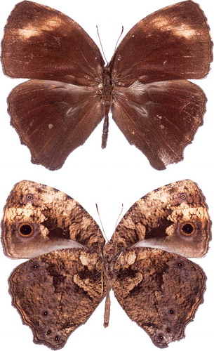
Fig. 6. Collection locations of morphologically investigated male specimens of B. mandanes (white squares), B. collinsi (black circles), and B. kenia (white circles). For more information about the total estimated distribution of the species see main text.

Fig. 7. Central African samples locations (generally verified through voucher photos) for the three species in the dorothea-complex: B. dorothea (white squares), B. moyses (grey diamonds), and B. jefferyi (black circles). Most locations in Gabon are sourced from Vande weghe (2010) while remaining data generally acquired from photos of voucher specimens in the collections of ABRI and MRAC. Some additional data are taken from fieldwork notes and photos by the authors and collaborators. The distribution of B. dorothea extends further to the west throughout all forested areas of West Africa (not shown), but in this region the two other species are fully absent.

Condamin, M. (1973). Monographie du genre Bicyclus (Lepidoptera Satyridae) [Monograph of the genus Bicyclus (Lepidoptera Satyridae)]. Dakar: IFAN-Dakar.

 Google Scholar

Vande weghe, G. (2010). Les papillons du Gabon. [Butterflies of Gabon]. Libreville: Wildlife Conservation Society.

 Google Scholar