Bernal’s road to random packing and the structure of liquids

Figures & data

Figure 1 The X-ray diffraction pattern of water compared with those predicted by Bernal’s quartz-like model, taken from a draft of the original 1933 paper [3].

Figure 2 The radial distribution function of Morrell and Hildebrand’s densest model (lower panel) compared with the experimental function for liquid mercury (top panel). Reprinted with permission from Morrell and Hildebrand [17]. Copyright 1936, American Institute of Physics.

Figure 3 The radial distribution function of Alder et al.’s densest Monte Carlo-computed hard sphere assembly. Reprinted with permission from Alder et al. [20]. Copyright 1955, American Institute of Physics.

Figure 4 Bernal building his first simple liquid model in his office.

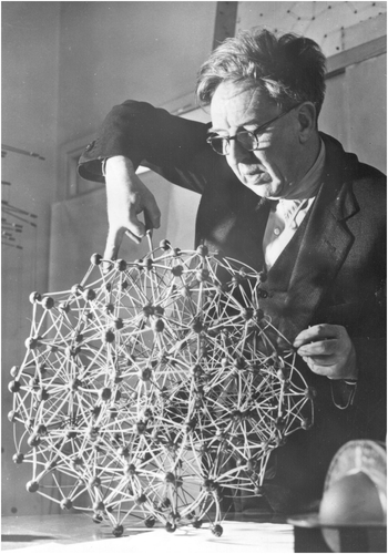
Figure 5 (colour online) (a) Magnetic sphere arrangement used to build irregular coordination models. (b) An example of an irregular coordination arrangement together with the equivalent Voronoi polyhedron. Reprinted by courtesy of the Royal Institution of Great Britain from Proc. Roy. Instn. 37 (1959) p.373.

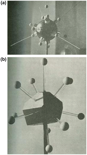
Figure 6 An exposed surface of the compressed plasticene sphere assembly.

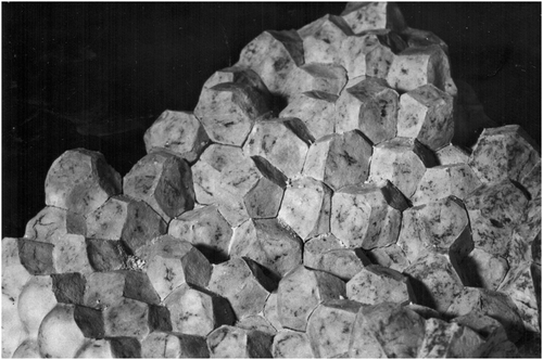
Figure 7 (colour online) (a) Bernal ‘crazy fishing’, with (b) the ball-and-spoke model constructed from the resulting high density arrangement of the hanging balls in (a). Reprinted by courtesy of the Royal Institution of Great Britain from Proc. Roy. Instn. 37 (1959) p.385.

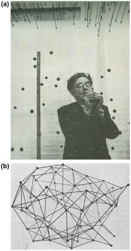
Figure 8 The radial distribution function of Bernal’s computer-constructed random hard sphere model, together with that of the subsequently ‘squeezed’ densified model, compared to that of liquid lead. Reprinted by permission from Macmillan Publishers Ltd.: Nature 185 (1960) 68, copyright 1960.

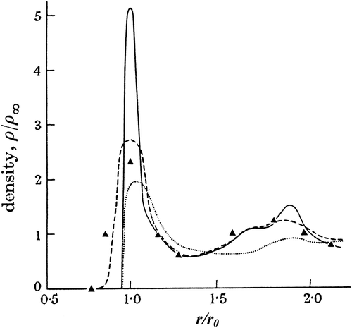
Figure 9 The five ‘canonical holes’ identified by Bernal in random sphere packings.

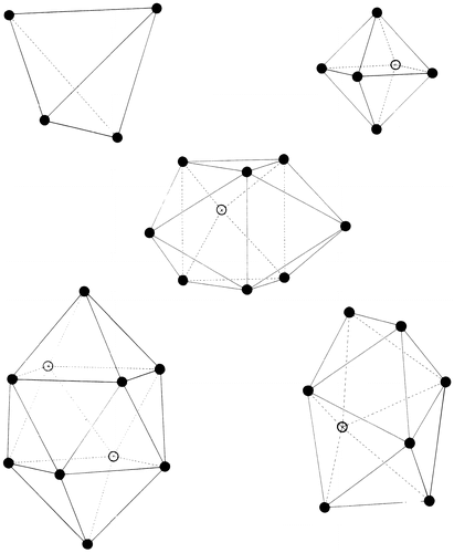
Figure 10 The ‘paint’ method of marking (left) close and (right) near contacts between spheres. Reprinted by permission from Macmillan Publishers Ltd.: Nature 188 (1960) 910, copyright 1960.

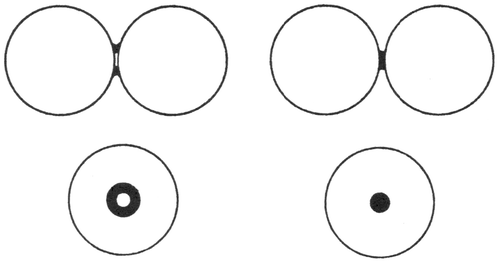
Figure 11 Part of a random packing of steel balls taken from a paint-fixed model.

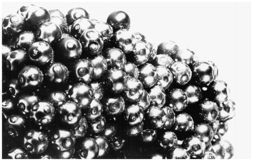
Figure 12 (colour online) The first expanded ball-and-spoke model built using the sphere coordinates measured from a paint-fixed random packing of steel spheres.

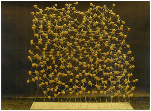
Figure 13 Looking down part of a collineation in an expanded ball and spoke model.

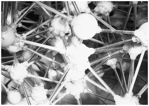
Figure 14 The experimental radial distribution function of liquid argon compared with those predicted from both the random packing models of Scott and Bernal.

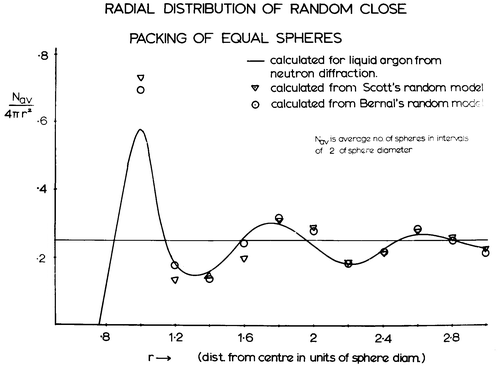
Figure 15 Building and measuring the large hard sphere model. (a) One of the two hemispherical surfaces used to suppress any crystallization at the surface; (b) the sample after binding with rubber strip; (c) the converted toolmaker’s microscope used to measure the sphere coordinates with the sample towards the end of the measurements; (d) a close-up of an exposed plane of the model.

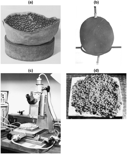
Figure 16 The radial distribution function of the large model at two different resolutions. First published in [35].

Figure 17 The distribution of edges per face of the Voronoi polyhedra elucidated from Monte Carlo simulations of crystalline argon at three temperatures up to the melting point, of liquid argon just above the melting point, together with that of the random hard sphere packing and two Monte Carlo simulations of the liquid using ‘hardened’ potentials. First published in [40].

Figure 18 The radial distribution functions of Monte Carlo simulations of crystalline and liquid argon, of the liquid using ‘hardened’ potentials, together with that of the random hard sphere packing. First published in [40].

J.D. Bernal and R.H. Fowler, J. Chem. Phys. 1 (1933) p.515.

 Web of Science ®Google Scholar

W.E. Morrell and J.H. Hildebrand, J. Chem. Phys. 4 (1936) p.224.

 Google Scholar

B.J. Alder, S.P. Frankel and V.A. Lewinson, J. Chem. Phys. 23 (1955) p.417.

 Web of Science ®Google Scholar

J.L. Finney, Proc. R. Soc. Lond. Ser. A 319 (1970) p.479.

 Web of Science ®Google Scholar

J.L. Finney, Proc. R. Soc. Lond. Ser. A 319 (1970) p.495.

 Web of Science ®Google Scholar