Concise review: aerodynamic noise prediction methods and mechanisms for wind turbines

Figures & data

Figure 1. Methods for computational aeroacoustics (Wagner, Hüttl, and Sagaut 2007).

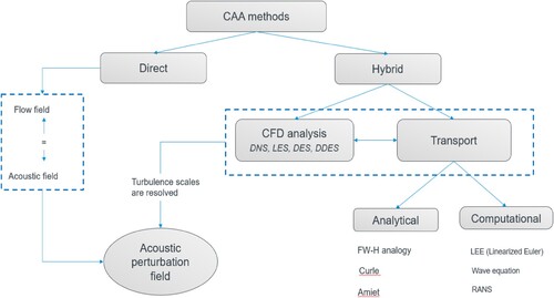
Figure 2. Relation between the CAA methods, acoustic analogies and prediction of acoustic field.

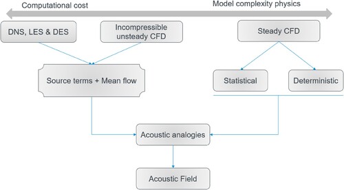
Figure 3. Interpretation of FW-H acoustic analogy in terms of source, observer regions and overlapping envelope surrounding the source and observer.

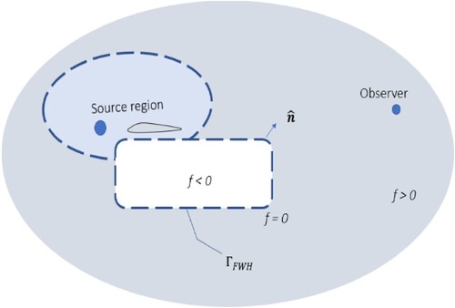
Figure 4. Illustration of different types of noise sources according to flow conditions.

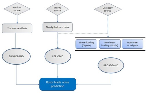
Table 1. General and wind turbine noise regulation standards and thresholds in different countries (Bhargava and Samala 2019a).

Country	Lp-d	Lp-n	ΔLpd-n	Regulation
India
Industrial zone	75	70	5	CPCB – 1993
Commercial zone	65	55	10
Residential zone	55	45	10
Special zone	50	35	15
China				GB 12523-2011^ϯ
Industrial zone	65	55	10	GB 12348-2008*
Traffic zone				GB 22337-2008^×
Road	70	55	15
Railway	70	60	10	CCAR – 36
Aircraft*	80	74	6
Residential zone
Plane	60	50	10
Mixed	55	45	10
Special zone	50	40	10
Germany	40	35	5	See Bastasch et al. (2006) ETSU-R-97
Denmark^+	44 @ 8 m/s; 42 @ 6 m/s
Canada/US	40–51 dB(A) 43 dB(A) + 5 dB (A) at evening; + 10 dB (A) at night 35/40 dB(A) + 5 dB(A) at night
UK
Australia

Noise metrics: L_pA = Aweighted perceived noise level; L_pd = Day time level; L_pd = Night time level; L_pd = Average of day and night time level; L_Aeq = A weighted equivalent continuous level; L₉₀, L₁₀ refers to background noise levels with 10% and 90% exceedance in measured data.

ϮConstruction.

×Community.

*Hong Kong international airport.

Figure 5. Resultant amplitude modulation of signal, f with a phase angle of 90° obtained using superimposing carrier signal (f_c = 50 Hz, A_c = 1), and modulation signal, f_m at modulation index, m = 0.9.

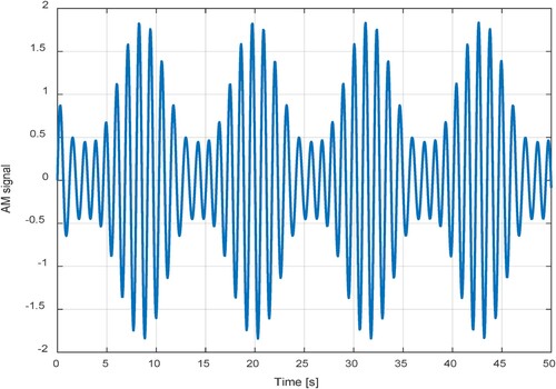
Figure 6. (a) Flow-induced noise sources from an aerofoil (Bhargava and Samala 2019b). (b) Illustration of wind turbine blade length (Bhargava and Samala 2019a).

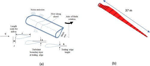
Figure 7. Illustration of sound pressure level varying with harmonic number, n, at wind speed of 13.5 m/s compared to experiment data measured downwind at distance of ∼100 m for (Δf = 0.25 Hz).

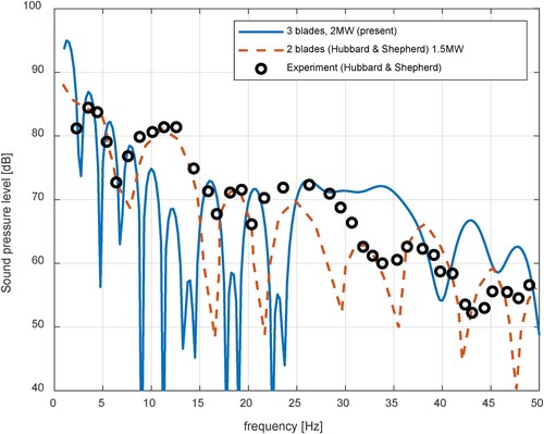
Figure 8. Experimental data for NACA 0012 aerofoil self-noise recorded in a wind tunnel for different test configurations (Sabat et al.).

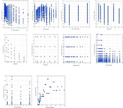
Table 2. Statistical descriptors for the aerofoil self-noise data (Viterna 1981).

Parameter	Mean	Std deviation	Min	Max	25%	50%	75%
Frequency (Hz)	2886.38	3152.57	200	20,000	800	1600	4000
Angle of attack (deg)	6.782	5.918	0	22.2	2.0	5.4	9.9
Chord length (m)	0.1365	0.0935	0.0254	0.3048	0.1016	0.1016	0.2286
Free stream velocity (m/s)	50.86	15.572	31.7	71.3	39.6	39.6	71.3
SPL (dB)	124.835	6.898	103.380	140.987	120.191	125.721	129.995

Table 3. Summary of past research findings related to aerofoil self-noise prediction methods.

Year	Author(s)	Summary/finding(s)	Source
1973, 1976	Paterson et al (1973), Paterson and Amiet (1976)	Conducted an experiment study on tonal noise characteristic which correlated boundary layer stability using boundary layer thickness and periodic vortex shedding frequencies. Formulated a theoretical model for surface pressure which can predict the far field noise based on inflow turbulence parameters and also validated the model with experiment data measured on 23 cm chord NACA 0012 aerofoil.	Journal of Aircraft (Paterson et al. 1973) NASA report, CR-2733
1974	Tam	Studied tonal noise using wind tunnel experiments and highlighted that self-excited aeroacoustic feedback loop is caused due to wake instabilities in laminar boundary layer from pressure side of aerofoil. Transient oscillations of acoustic waves in far field were found to dependent on near field pressure perturbations.	Journal of Acoustical Society of America (Tam 1974)
1981	Shlinker and Amiet	Studied helicopter rotor noise prediction techniques based on turbulence boundary layer theory and developed analytical formulations using spanwise flow coherence correlations on blades. Showed that spanwise flow coherence relations strongly influenced far field rotational noise prediction.	NASA CR 3470 (Schlinker and Amiet 1981)
1983	Arbey and Bataille	Found that broadband noise spectra for laminar flows are attributed to edge diffraction of T-S waves instabilities at leading edge to produce discrete tones. Investigated the self-excited aeroacoustic feedback loop and position of maximum velocity point along chord length of aerofoil.	Journal of Fluid Mechanics (Arbey and Bataille 1983)
1999	Nash, MacAlpine et al.	Investigated tonal noise characteristics based on boundary layer flow separation mechanisms that couple acoustic waves travelling upstream of trailing edge of aerofoil along with T-S wave instabilities downstream of chord. This is based on work proposed by Tam (1974)	Journal of Sound and Vibration (McAlpine, Nash, and Lowson 1999)
1989	Brookes, Pope and Marcolini	Developed the semi empirical noise model for prediction of aerofoil self-noise mechanisms using measured wind tunnel test data and curve fitting techniques. Used aerofoils of chord length up to 60 cm in wind tunnel tests and validated SPL spectra at Mach numbers ranging from 0.1 to 0.6.	NASA reference publication 1218 (Brooks, Pope, and Marcolini 1989)
2003	Moriarty and Migliore	Extended the BPM model and investigated aerofoil self-noise mechanisms for small-scale wind turbines and aerofoils. Validation for sound pressure were found to deviate by 6 dB for high Re flows compared to predicted results.	NREL Technical Report (Moriarty and Migliore 2003) https://www.nrel.gov/
2007	Oerlemans	Performed parametric study on optimum microphone array locations that were found to reduce the measured SPL by 3–6 dB for various flow configurations. Used phased microphone arrays method for detection of noise sources from aircrafts and wind turbines.	Journal of Sound and Vibration (Oerlemans, Sijtsma, and Lopez 2007)
2009	Moreau et al.	Found that stall phenomenon influenced the measured far field SPL by 6 dBA in low-frequency region for a series of NACA four-digit aerofoils. Also concluded that SPL spectra is sensitive to changes in Angle of Attack (AoA) caused due to turbulence anisotropy.	30th AIAA aero-acoustics conference (Moreau, Roger, and Christophe 2009)
	Kingan and Pearse	Developed a theoretical model using Orr–Sommerfeld linear stability equation for laminar boundary layer on leading edge of flat plate. Also compared the results with BPM model, Arbey and Bataille test model. This work is based on the work done by Shapiro (1977)	Journal of Sound and Vibration (Kingan and Pearse 2009)
2016	Wei et al.	Investigated the optimised aerofoil designs using different CAA-based solvers for low noise aerofoil design analysis. Also proposed a new spectral shape function for trailing edge bluntness noise model based on original BPM model.	IntechOpen book: Wind turbines-design, control and applications (Zhu, Shen, and Sorensen 2016)
2020	Carpio et al.	Assessed the noise abatement techniques for NACA 0018 aerofoil (chord length of 20 cm) using optimal solid and perforated trailing edge 3D printed inserts. Approximately 20 dB noise reduction was achieved using moderate permeability, however, an ordered pore arrangement of inserts produced loud tones due to vortex shedding from trailing edge of aerofoils.	Journal of Sound and Vibration (Caprio et al. 2020)
2021	Moreau Daniel	Conducted experiment study of flow induced noise for wall-mounted 3D aerofoils. Trailing edge and tip vortex formation noise sources were analysed primarily for a series of NACA symmetric aerofoils. Different aspect ratios, thicknesses, surface porosities and tip shapes were considered in the study	Proceedings of Acoustics 2021, Wollongong (Moreau 2021)

Figure 9. (a) One-third octave band frequency spectra of overall sound pressure level (with and without tip noise contribution) from NACA 0012 airfoil using BPM method having a chord length of 16cm and validated with 2D and 3D experiment wind tunnel data at U = 71.3 m/s and Angle of attack, α = 10° (Brooks, Pope, and Marcolini 1989). (b) Computed tip noise predicted from BPM model for square, round and sharp tip geometries for a 2MW wind turbine blade.

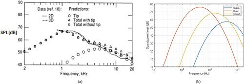
Figure 10. Self-noise spectra turbulent boundary layer trailing edge noise of NACA 0012 computed using BPM method at free stream velocity, U = 65 m/s (a) at 8° AOA for chord lengths of 1.5, 0.8 and 0.5 m (b) for chord length of 0.5 m at 2°, 4° and 8° angle of attack (Bhargava and Samala 2019b; Bhargava and Samala 2019a; Bhargava, Samala, and Anumula 2019).

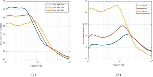
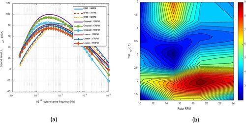
Figure 11. Comparison of (a) sound pressure (L_Aeq) and power (L_w) level difference with experiment data of Van den Berg (2006) for different rotational speeds of three-bladed turbine (b) sound pressure (L_Aeq) predicted using 1x, 1.2x and 2x logarithmic velocity profile expressions for different wind speeds measured at 10 m height with experiment data of Van den Berg (2006).

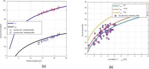
Figure 12. (a) Turbulent boundary layer trailing edge noise computed using BPM, Lowson and Grosveld methods as function of rotor RPM (Bhargava and Samala 2019a). (b) Standard error of sound pressure (dBA) between BPM, Lowson and Grosveld methods at U = 8 m/s for increasing rotational speed in RPM.

Wagner, C., T. Hüttl, and P. Sagaut, eds. 2007. “Introduction.” In Cambridge Aerospace Series, 1–23. London: Cambridge University Press.

 Google Scholar

Bhargava, V., and R. Samala. 2019a. “Acoustic Emissions from Wind Turbine Blades.” Journal of Aerospace Technology and Management. doi:10.5028/jatm.v11.1071.

 Web of Science ®Google Scholar

Bastasch, M., J. van Dam, B. Sondergaard, and A. Rogers. 2006. “Wind Turbine Noise – An Overview.” Journal of Canadian Acoustical Association 34 (2): 7–16.

 Google Scholar

Bhargava, V., and R. Samala. 2019b. “Effect of Boundary Layer on Broadband Noise from Wind Turbine Blades.” Journal of Aerospace Technology and Management, doi:10.5028/jatm.v11.1045.

 Web of Science ®Google Scholar

Viterna, L.A. 1981. “The NASA LeRC Wind Turbine Sound Prediction Code, 2nd DOE/NASA Wind Turbine Dynamics Workshop.” Report no: TM-81737/20366-1.

 Google Scholar

Paterson, R.W., P.G. Vogt, M.R. Fink, and C.L. Munch. 1973. “Vortex Noise of Isolated Airfoils.” Journal of Aircraft 10: 296–302. doi:10.2514/3.60229.

 Google Scholar

Paterson, R.W., and R.K. Amiet. 1976. Acoustic Radiation and Surface Pressure Characteristics of an Airfoil due to Incident Turbulence, NASA Report, CR-2733.

 Google Scholar

Tam, C.K.W. 1974. “Discrete Tones of Isolated Airfoils.” Journal of Acoustical Society of America 55: 1173–1177. doi:10.1121/1.1914682.

 Web of Science ®Google Scholar

Schlinker, R., and R.K. Amiet. 1981. “Helicopter Rotor Trailing Edge Noise.” NASA CR 3470.

 Google Scholar

Arbey, H., and J. Bataille. 1983. “Noise Generated by Airfoils Placed in Uniform Laminar Flow.” Journal of Fluid Mechanics 134: 33–47. doi:10.1017/S0022112083003201.

 Web of Science ®Google Scholar

McAlpine, A., E.C. Nash, and M.V. Lowson. 1999. “On the Generation of Discrete Frequency Tones by the Flow Around an Airfoil.” Journal of Sound and Vibration 222: 753–779. doi:10.1006/jsvi.1998.2085.

 Web of Science ®Google Scholar

Brooks, T.F., D.S. Pope, and M.A. Marcolini. 1989. Airfoil Self Noise and Prediction. NASA Reference Publication 1218. https://ntrs.nasa.gov/archive/nasa/casi.ntrs.nasa.gov/19890016302.pdf.

 Google Scholar

Moriarty, P., and P. Migliore. 2003. “Semi Empirical Aero-Acoustic Noise Prediction Code for Wind Turbines.” Technical Report. http://citeseerx.ist.psu.edu/viewdoc/download?doi=10.1.1.197.1153&rep=rep1&type=pdf.

 Google Scholar

Oerlemans, S., P. Sijtsma, and M.B. Lopez. 2007. “Location and Quantification of Noise Sources on a Wind Turbine.” Journal of Sound and Vibration 299 (5), doi:10.1016/j.jsv.2006.07.032.

 Web of Science ®Google Scholar

Moreau, S., M. Roger, and J. Christophe. 2009. “Flow Features and Self-Noise of Airfoils Near Stall or in Stall.” 30th AIAA Aeroacoustics Conference. doi:10.2514/6.2009-3198.

 Google Scholar

Shapiro, P.J. 1977. “The Influence of Sound Upon Laminar Boundary Layer Instability.” Report No: 83458-83560-1.

 Google Scholar

Kingan, M.J., and J.R. Pearse. 2009. “Laminar Boundary Layer Instability Noise Produced by an Aerofoil.” Journal of Sound and Vibration 322: 808–828. doi:10.1016/j.jsv.2008.11.043.

 Web of Science ®Google Scholar

Zhu, W.J., Wen Zhong Shen, and J.N. Sorensen. 2016. “Low Noise Airfoil and Turbine Design.” In Wind Turbines-Design, Control and Applications, 55–72. Intech Open. doi:10.5772/63335.

 Google Scholar

Caprio, A.R., F. Avallone, D. Ragni, M. Snellen, and S. van der Zwaag. 2020. “Quantitative Criteria to Design Optimal Permeable Trailing Edges for Noise Abatement.” Journal of Sound and Vibration 485. doi:10.1016/j.jsv.2020.115596.

 Web of Science ®Google Scholar

Moreau, D. 2021. “Flow Induced Noise Regimes for Three-Dimensional Airfoil.” Proceedings of Acoustics 2021, Wollongong, NSW, Australia.

 Google Scholar

Bhargava, V., R. Samala, and C. Anumula. 2019. “Prediction of Broadband Noise from Symmetric and Cambered Airfoils.” INCAS Bulletin, doi:10.13111/2066-8201.2019.11.1.3.

 Google Scholar

Van den Berg, G.P. 2006. “The Sound of High Winds: The Effect of Atmospheric Stability on Wind Turbine Sound and Microphone Noise.” Doctoral thesis, University of Groningen.

 Google Scholar