Figures & data
Figure 1. World total final consumption (TFC) by fuel (Mtoe).
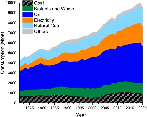
Figure 2. Historical installed capacity by fuel type in Colombia.
Adapted from (UPME Citation2023).
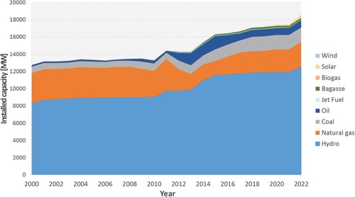
Figure 3. LCOE of different types of technology in the period 2020–2022.
Adapted from (NREL Citation2022).
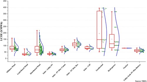
Figure 4. Schematic of the hybrid system in HOMER.
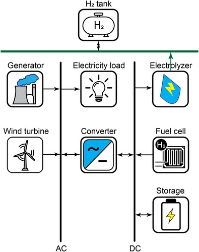
Figure 5. HOMER algorithm scheme.
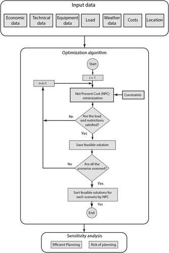
Figure 6. Community load profile, including workdays and weekends.
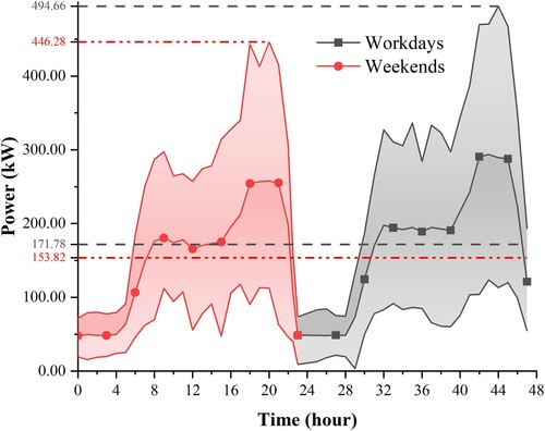
Figure 7. Average speed wind map from Colombia in February (left) and October (right) (m/s).
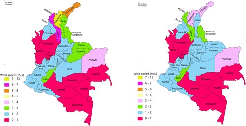
Figure 8. Wind speed (m/s) in the municipality of Uribia-Guajira.
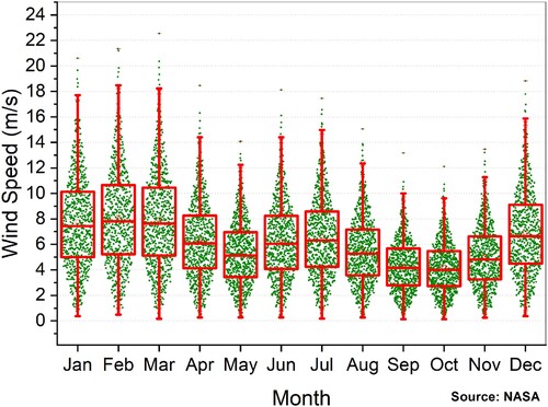
Figure 9. XANT M-24-ETR power curve.
Data adapted from (XANT Citation2017).
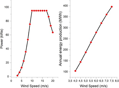
Table 1. Equipment considered in the analysis.
Table 2. Search space during optimisation.
Table 3. Result of cost minimisation for the scenario d = 12%, i = 13.44% and average wind speed 4 m/s.
Table 4. Result of cost minimisation for the scenario d = 12%, i = 13.44% and average wind speed 6.2 m/s.
Table 5. Result of cost minimisation for the scenario d = 12%, i = 13.44% and average wind speed 7.5 m/s.
Figure 10. Result of the cost minimisation for the scenario d = 12%, i = 13.44% (a, b, c), d = 17%, and i = 20.44% (d, e, f), with average wind speed 4 m/s (a, d), 6.2 m/s (b, e), and 7.5 m/s (c, f).
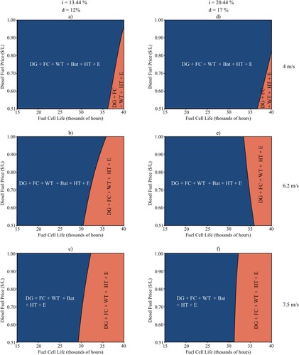
Figure 11. Cash flow for the selected scenario and configuration.
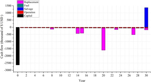
Table 6. Summary of the costs associated with the recommended system (values in thousands of dollars).
Figure 12. Average monthly performance during one year of operation of the selected system.
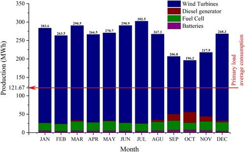
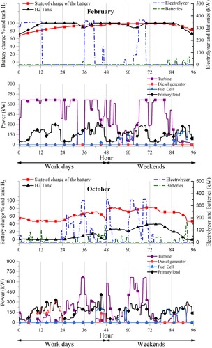
Figure 13. Performance hour-by-hour of the selected system during February and October.