Figures & data
Figure 1. A scattering of some of the 253 harvested sites seen in the rugged terrain at landscape level (red polygons, left) and a close-up illustrating how one harvested site is made up of multiple DMUs, each shown in a different gray tone (right). Spatially, a DMU represents the area felled by a harvester on any single day. The dataset constituted 643 such DMUs
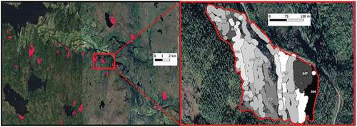
Figure 2. Examples of how stand shape is quantified by the isoperimetric ratio, which is the ratio between stand area and the area of a circle with the same perimeter; (a) a roughly circular stand with isoperimetric ratio = 0.81, and (b) an elongated stand with isoperimetric ratio = 0.13. The points represent the position of the harvester at felling, while the stand polygon is created by buffering these points by 10 m
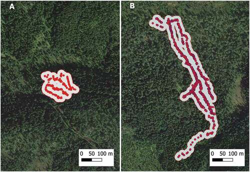
Table 1. Variables description
Table 2. Summary statistics for the ground conditions (Topography), the machine (Machine related), the site (Site/Forest parameters), and the output produced (Products/Assortments)
Figure 3. Example of actual route of a harvester vs. the computed minimal route for one harvest site (sparse forest cover, area of DMU is 24.86 ha). The connecting green line shows the order in which trees were cut and the red connecting line shows the order in which the trees should have been cut to minimize the total traveling distance
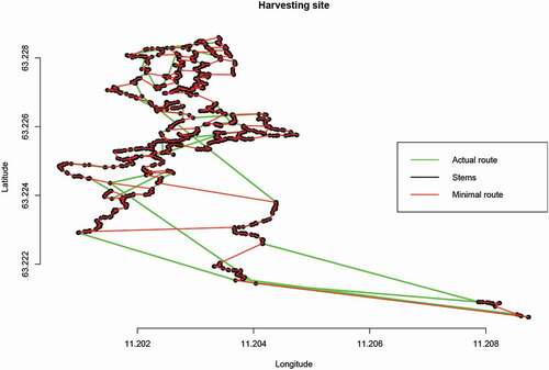
Figure 4. Histogram of actual/minimal travel distance (m)
Figure 5. Histogram of inefficiency scores β.
Figure 6. Boxplot of slacks in inputs (βgx)
Figure 7. Nonparametric regression of (actual/minimal) travel distance on inefficiency scores
Table 3. Regression results with site level variables in Z variables but not in regression
Figure 8. Nonparametric regression of tree density on (actual/minimal) travel distance (m)