Tensile forces and deflections on skylines of cable yarders: comparison of measurements with close-to-catenary predictions

Figures & data

Table 1. Support positions in the length profile. IS: intermediate support; TS: tail spar; z_cs: z-coordinate of the cable shoe (= z_bs,i + h_s,i); x_s,i: x-coordinate of the cable shoe; w_i: width of span i; z_b,si: vertical distance from the coordinate origin to the bottom of the support i (Figure 1); h_s,i: height of cable shoe i from ground (Figure 1). BW: Buriwand; KB: Koebelisberg; BL2 and BL3: Banzenloecher Lines 2 and 3

Cable road		Yarder Tower	IS 1	IS 2	TS	Anchor
BW	zcs [m]	12	168.1	216.9	255.6	260.9
	xs [m]	0	241.14	326.24	391.78	421.02
		Yarder Tower	IS	Anchor
KB	zcs [m]	11.5	−27.4	−128.2
	xs [m]	0	88.63	371.87
		Yarder Tower	IS	TS	Anchor
BL2	zcs [m]	11.5	98.5	115.3	114.3
	xs [m]	0	345.52	407.42	439.40
		Yarder Tower	IS 1	IS 2	TS	Anchor
BL3	zcs [m]	9.4	50.5	94.4	131.6	129.7
	xs [m]	0	170.52	341.23	471.69	506.68

Table 2. Span dimensions. w: span width; h: span height; BW: Buriwand; KB: Koebelisberg; BL2 and BL3: Banzenloecher Lines 2 and 3

		Span Number
Cable road		1	2	3	4
BW	w [m]	241.14	85.10	65.54	29.24
	h [m]	156.11	48.83	38.63	5.29
KB	w [m]	88.63	283.24
	h [m]	−38.93	−100.75
BL2	w [m]	345.52	61.90	31.98
	h [m]	86.96	16.81	−0.92
BL3	w [m]	170.52	170.71	130.46	34.99
	h [m]	40.68	43.93	37.14	−1.88

Figure 1. Cable road properties.

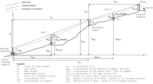
Table 3. Position and properties of the measurement points. x_m: horizontal distance from the head spar to the measurement point [m]; z_m: vertical distance from the bottom of the head spar to the measurement point [m]; z_{ch_m}: vertical distance from the bottom of the head spar to the corresponding height of the span chord at the measurement point [m]; d_{g_ch_m}: distance span-chord to ground [m] (= z_{ch_m –}z_m). BW: Buriwand; KB: Koebelisberg; BL2 and BL3: Banzenloecher Lines 2 and 3

Cable road	Span number	1	2	3
BW	xm [m]	122.50	283.80	365.80
	zm [m]	66.78	177.44	228.59
	zch_m [m]	91.30	192.58	240.22
	dg_ch_m [m]	24.52	15.14	11.63
KB	xm [m]	45.00	207.64
	zm [m]	−22.68	−111.50
	zch_m [m]	−8.27	−69.73
	dg_ch_m [m]	14.41	41.77
BL3	xm [m]	85.40	250.00	406.40
	zm [m]	9.30	45.53	92.87
	zch_m [m]	29.77	70.95	112.95
	dg_ch_m [m]	20.47	25.42	20.08
BL2	xm [m]	130.47	375.71
	zm [m]	11.25	89.44
	zch_m [m]	44.34	106.70
	dg_ch_m [m]	33.09	17.26

Table 4. Rope and machine properties. BW: Buriwand; KB: Koebelisberg; BL2 and BL3: Banzenloecher Lines 2 and 3

Factor	Unit	BW	KB	BL2	BL3
Yarder type		Syncrofalke – 4 t (Mayr- Melnhof)	KMS 12 (Konrad)	K507 (Koller)	K507 (Koller)
Carriage type		Sherpa U4 XL (Mayr-Melnhof)	Liftliner (Konrad)	Hansliner (in-house construction Abächerli AG)	Skytiger ST 50 (Seik)
Carriage weight	kg	720	790	850	1200
Skyline type		Styria Forst 2 (Haase)	Python Super (Jakob) 8S, 22 mm	Performance, F-30, (Teufelberger) 20.5 mm	Performance, F-30, (Teufelberger) 20.5 mm
Skyline minimum breaking force	kN	430.95	442.80	453.00	453.00
Skyline E-modulus (range, used for sensitivity analysis)	kN mm^−2	100–130	95–105	95–105	95–105
Skyline E-modulus (used for analysis)	kN mm^−2	115	100	100	100
Skyline self-weight	kN m^−1	0.0228	0.0223	0.0205	0.0205
Skyline diameter	mm	22	22	20.5	20.5
Skyline fill factor	[]	0.78	0.68	0.78	0.78
Mainline type		Teufelberger, F20	Teufelberger, FSS 2–619S 3AY, 12 mm	Teufelberger,F-20 (6x25) 12 mm	Teufelberger,F-20 (6x25) 12 mm
Mainline self-weight	kN m^−1	0.0072	0.0074	0.0073	0.0073

Figure 2. Weighed logs for load formation at the Buriwand (BW) cable road. The numbers on the logs indicate the weight of the single logs in tons [t]. Please note that both comma and point are used as a decimal point and that the 0.8 is upside-down (reads 8.0 but is 0.8 in reality) (photo: Leo Bont).

Table 5. Load (Q) of different load configurations (LC) at the different test sites. Load configuration LC1 was the carriage only, whereas LC2 to LC4 were composed of the carriage and different log combinations. BW: Buriwand; KB: Koebelisberg; BL2 and BL3: Banzenloecher Lines 2 and 3

Cable road	Carriage (LC1) [kN]	LC2 [kN]	LC3 [kN]	LC4 [kN]
BW	7.06	17.85	26.68	35.02
KB	7.75	18.15	25.41	32.67
BL2	8.34	12.56	19.42	30.31
BL3	11.77	22.66	29.53	33.75

Figure 3. Free body diagram of forces acting in the equilibrium equation of the carriage. (A) Situation for the Zweifel (1960) assumptions, in which the carriage is clamped onto the skyline. Zweifel (1960) includes the skyline tensile forces and the load Q_Z (carriage weight, load and mainline self-weight) in the equilibrium equation of the carriage. The equilibrium equation is as follows: Q_Z + V_S,L+ V_S,R = 0 and H_S,L = H_S,R. (B) Measured situation in which the carriage is held by the mainline. In this case, the skyline and the mainline/haulbackline tensile forces and the load Q_M (carriage-weight and load) are included in the equilibrium equation of the carriage. The equilibrium equation is as follows: Q_M + V_S,L+ V_S,R+ V_M,L+ V_M,R = 0 and H_S,L + H_M,L = H_S,R+ H_M,R.V_S: vertical component of the skyline tensile force, V_M: vertical component of the mainline tensile force, H_S: horizontal component of the skyline tensile force, H_M: horizontal component of the mainline tensile force, R: right, L: left.

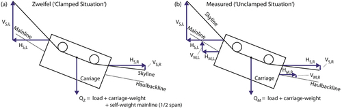
Table 6. Measured mounting tension for each project site. To measure the mounting tension, the unloaded carriage was located 1 m from the tower. The basic skyline tensile force (mounting tension) was measured anew each time a switch was made to a new span

	Measurement place [M = mountain, V = valley]	Mounting tension ($T_{0,E}$) [kN] (measured value of load cell before measurement in span)
Cable road		1	2	3
BW	M	83.48	80.64	79.46
KB	V	88.19	91.72
BL2	M	124.59	120.07
BL3	M	116.54	112.23	110.07

Figure 4. Sketch of the measurement layout. The ground clearance is calculated based on the distances and angles to the transponder and the skyline.

Figure 5. PAT load cell at the mountain anchor of the Buriwand (BW) cable road (photo: Fritz Frutig).

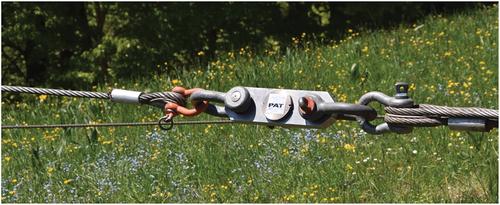
Figure 6. (A) Measured skyline tensile forces (T_MT) in the cable roads and spans for the different load configurations. The bottom end of each line indicates the mounting tension/pre-stress tensile force. (B) Absolute measured deflection (AMD) of the skyline [m], derived from the measured ground clearance, for the different load configurations and the respective spans. Cable road abbreviations: BW: Buriwand, KB: Koebelisberg, BL2 and BL3: Banzenloecher Lines 2 and 3.

Figure 7. (A) Differences between the measured skyline tensile force and the theoretical values (ΔT_ZM) [%]. The measured value serves as a reference. A positive ΔT value means that the theoretical skyline tensile forces are higher than the measured ones. Only loaded skyline configurations are displayed. (B) Differences between the theoretical (RTD) and the measured relative (RMD) skyline deflection for loaded situations (Δy_ZM,rel) [m]. A positive value means that the theoretical deflection values are higher than the measured ones. Cable road abbreviations: BW: Buriwand, KB: Koebelisberg, BL2 and BL3: Banzenloecher Lines 2 and 3.

Table 7. Root mean square error (RMSE), mean absolute error (MAE), mean absolute percentage error (MAPE) and root mean square error in percent (RMSE_P) for the skyline tensile force calculations compared with the measured values. The metrics were computed for each cable road separately and for all cable roads together (overall)

Cable road	RMSE [kN]	MAE [kN]	MAPE [%]	RMSE_P [%]
BL2	1.45	1.13	0.69	0.87
BL3	3.02	2.71	1.82	2.01
BW	8.25	5.86	4.65	6.07
KB	10.6	8.1	5.9	7.4
Overall	6.75	4.39	3.22	4.78

Figure 8. (A) Comparison of the differences in the skyline tensile forces (ΔT_ZM) [%] (theoretical vs. measured) and (B) the relative difference in deflection (Δy_ZM,rel) [m] (theoretical vs. measured) compared with the slope for each span. Cable road abbreviations: BW: Buriwand, KB: Koebelisberg, BL2 and BL3: Banzenloecher Lines 2 and 3.

Figure 9. Deflection of the unloaded skyline. Comparison of absolute measured deflection (AMD) and absolute theoretical deflection (ATD). Cable road abbreviations: BW: Buriwand, KB: Koebelisberg, BL2 and BL3: Banzenloecher Lines 2 and 3.

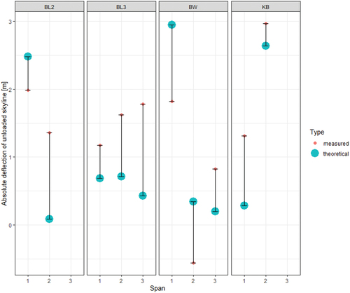
Table 8. Root mean square error (RMSE), mean absolute error (MAE), mean absolute percentage error (MAPE) and root mean square error in percent (RMSE_P) for the deflection calculations compared with the measured values. The metrics were computed for each cable road separately and for all cable roads together

Cable road	RMSE [m]	MAE [m]	MAPE [%]	RMSE_P [%]
BL2	0.32	0.26	4.89	5.42
BL3	0.56	0.49	7.48	8.64
BW	0.31	0.25	4.96	7.22
KB	0.60	0.55	8.99	10.49
Overall	0.47	0.39	6.55	8.14

Figure 10. Comparison of the differences in the skyline tensile forces (ΔT_ZM) [%] (theoretical vs. measured) and the relative difference in deflection (Δy_ZM,rel) [m] (theoretical vs. measured) with regression line for each cable road. Cable road abbreviations: BW: Buriwand, KB: Koebelisberg, BL2 and BL3: Banzenloecher Lines 2 and 3.

Figure 11. Absolute deflections for the loaded (loading configurations 1–4) and the unloaded skyline (loading configuration 0) for the approaches of Zweifel (1960) and Pestal (1961) and for the measured values (Meas). Cable road abbreviations: BW: Buriwand, KB: Koebelisberg, BL2 and BL3: Banzenloecher Lines 2 and 3.

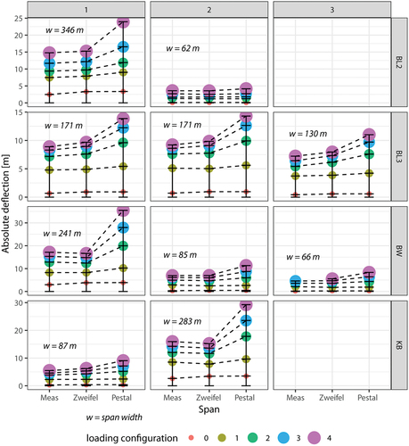
Figure 12. Sensitivity analysis for varying E-modulus (displayed for all load configurations). (A) Range for the difference between theoretical and measured skyline tensile force (ΔT_ZM) [%]. (B) Range for the relative difference between theoretical and measured deflection (Δy_ZM,rel) [m]. In A, the upper bound of the “error bar” represents the highest E-modulus (105 for BL2, BL3 and KB; 130 for BW) [kN mm⁻²], whereas the lower bound represents the lowest E-modulus (95; 100) [kN mm⁻²]. The point in the center indicates the mean of the range (100; 115) [kN mm⁻²]. In B, the displayed E-modulus values are exactly the other way around: the upper bound of the “error bar” represents the lowest E-modulus. Cable road abbreviations: BW: Buriwand, KB: Koebelisberg, BL2 and BL3: Banzenloecher Lines 2 and 3.

Raw measurement data. The deflection measurement data were derived from ground clearance measurements; (* = not measured at top-anchor, derived from bottom-anchor measured value according to Equation 1(1) $T_{0,S}=T_{0,E}-\mathrm{\Delta }{z}_{E,S}\ast q_S$(1) )

					Skyline tensile force			Deflection (difference from span chord to skyline at measurement point)
Cable road	Span	Load configuration	Load (Q)	Mounting tension (T_0,S)	Zweifel (top-anchor, TZT)	Meas. (top-anchor, TMT)	Meas. (bottom-anchor)	Zweifel (ATD)	Pestal	Meas. (AMD)	Zweifel/Pestal (unloaded skyline)(ATDUL)	Measured (unloaded skyline) (AMDUL)
			[kN]	[kN]	[kN]	[kN]		[m]	[m]	[m]	[m]	[m]
BW	1	1	7.063	77.82	102.67	100.16		8.26	10.25	7.12	2.95	1.82
BW	1	2	17.85	77.82	131.92	123.90		12.42	19.98	11.72	2.95	1.82
BW	1	3	26.68	77.82	154.11	141.26		14.81	27.94	14.22	2.95	1.82
BW	1	4	35.02	77.82	173.61	154.02		16.63	35.46	16.02	2.95	1.82
BW	2	1	7.063	74.98	86.39	86.82		2.47	2.65	1.94	0.35	−0.56
BW	2	2	17.85	74.98	102.33	101.04		4.70	5.99	4.04	0.35	−0.56
BW	2	3	26.68	74.98	116.51	115.56		6.01	8.73	5.24	0.35	−0.56
BW	2	4	35.02	74.98	129.70	122.63		6.98	11.32	6.04	0.35	−0.56
BW	3	1	7.063	73.80	83.71	83.48		1.80	1.89	2.73	0.20	0.83
BW	3	2	17.85	73.80	96.84	93.20		3.61	4.38	4.23	0.20	0.83
BW	3	3	26.68	73.80	109.27	101.34		4.70	6.42	5.23	0.20	0.83
BW	3	4	35.02	73.80	120.96			5.53	8.34		0.20	0.83
KB	1	1	7.75	91.30	96.68	98.27*	95.16	2.31	2.45	3.31	0.29	1.31
KB	1	2	18.15	91.30	110.61	112.98*	109.87	4.30	5.21	4.91	0.29	1.31
KB	1	3	25.41	91.30	121.61	123.09*	119.98	5.36	7.15	5.61	0.29	1.31
KB	1	4	32.67	91.30	132.68	135.54*	132.44	6.24	9.08	6.51	0.29	1.31
KB	2	1	7.75	94.83	116.27	109.06*	105.95	7.85	9.63	8.87	2.64	2.97
KB	2	2	18.15	94.83	145.15	131.62*	128.51	11.65	17.83	12.37	2.64	2.97
KB	2	3	25.41	94.83	164.33	146.34*	143.23	13.59	23.55	14.57	2.64	2.97
KB	2	4	32.67	94.83	182.46	164.48*	161.37	15.21	29.28	16.27	2.64	2.97
BL2	1	1	8.339	122.48	143.23	145.19		7.90	9.02	6.99	2.48	1.99
BL2	1	2	12.56	122.48	153.73	155.19		9.72	11.89	8.89	2.48	1.99
BL2	1	3	19.42	122.48	171.23	173.64		12.18	16.55	11.19	2.48	1.99
BL2	1	4	30.31	122.48	198.36	196.20		15.26	23.94	14.29	2.48	1.99
BL2	2	1	8.339	117.97	122.34	122.43		1.21	1.23	2.56	0.09	1.36
BL2	2	2	12.56	117.97	124.84	124.59		1.73	1.80	2.96	0.09	1.36
BL2	2	3	19.42	117.97	130.03	129.88		2.51	2.71	3.96	0.09	1.36
BL2	2	4	30.31	117.97	140.34	139.79		3.57	4.17	4.86	0.09	1.36
BL3	1	1	11.77	114.09	129.02	130.08		4.91	5.44	5.27	0.69	1.17
BL3	1	2	22.66	114.09	146.83	148.33		7.60	9.61	7.67	0.69	1.17
BL3	1	3	29.53	114.09	158.64	160.69		8.95	12.23	8.77	0.69	1.17
BL3	1	4	33.75	114.09	165.89	166.77		9.68	13.85	9.37	0.69	1.17
BL3	2	1	11.77	109.77	125.26	128.51		5.03	5.62	6.02	0.71	1.62
BL3	2	2	22.66	109.77	143.51	147.15		7.75	9.92	8.52	0.71	1.62
BL3	2	3	29.53	109.77	155.45	158.92		9.10	12.63	9.52	0.71	1.62
BL3	2	4	33.75	109.77	162.76	166.77		9.84	14.30	10.12	0.71	1.62
BL3	3	1	11.77	107.61	119.98	121.64		3.87	4.22	5.08	0.43	1.78
BL3	3	2	22.66	107.61	135.29	137.34		6.17	7.59	6.78	0.43	1.78
BL3	3	3	29.53	107.61	145.73	149.11		7.33	9.71	7.78	0.43	1.78
BL3	3	4	33.75	107.61	152.17	157.74		7.96	11.01	8.58	0.43	1.78

Figure A1. Residual plot for the random intercept model #1 (rim #1).

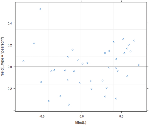
Figure A2. Residual plot for the random intercept model #2 (rim #2).

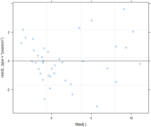
Figure A3. R command and summary model output for the random intercept model 1 (rim #1).Variables: y_norm_Delta: ‘difference in relative deflection’ (RTD - RMD) [m]; delta_T_perc: ‘diff. in skyline tensile force (STF)’(theor. STF – meas. STF) / meas. STF * 100 [%]; slope: ‘slope of the span’ []; Span_Width: ‘spanwidth’ [m]; Q:‘load’ [kN].

Figure A4. R command and summary model output for the random intercept model 2 (rim #2).

Figure A5. R command and summary model output for the simple linear regression model (lm #1).

Zweifel O. 1960. Seilbahnberechnung bei beidseitig verankerten Tragseilen. Schweiz Bauztg. 78:11.

 Google Scholar

Pestal E. 1961. Seilbahnen und Seilkräne für Holz- und Materialtransporte. Wien und München: Georg Fromme & Co.

 Google Scholar