A multi-objective optimization strategy for timber forwarding in cut-to-length harvesting operations

Figures & data

Figure 1. Schematic description of forwarding work at a CTL harvesting site.

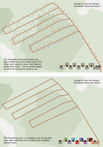
Figure 2. Illustration of the effect of the number of assortments on forwarder unloading time.

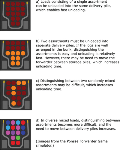
Figure 3. The algorithm used for estimating the sizes and positions of assortment-specific log piles created by the harvester. The function “add neighbors” is separately expanded on the right.

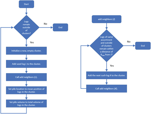
Figure 4. Example of estimating pile positions from harvester data. Squares represent the recorded position of the harvester cabin when felling a stem. This position is recorded for all logs from that stem. Dots depict the positions of the logs, to which small random noise has been added for purely visual purposes in this image. Stars depict the final, estimated pile positions.

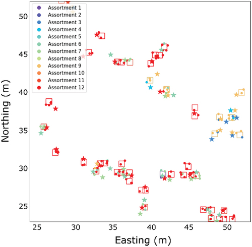
Table 1. Summary of the harvester data used in this work. The area of each system and the removal per hectare are estimates. The system used for producing the route optimization results presented in the Results section is highlighted with italics. DBH stands for diameter at breast height, std for standard deviation.

System	Type of harvest	Number of piles	Number of logs in a pile	Volume of piles (m^3)	Pile extent (m)	Mean DBH (mm)	Species distribution	Total volume of harvested timber (m^3)	Area (ha)	Harvested timber per hectare (m^3/ha)	Total number of assortments
1	Thinning	448	1 to 33, mean 4.6, std 5.1	0.010 to 2.0, mean 0.27, std 0.30	0.00 to 7.3, mean 0.53, std 1.0	144	79.7% pine, 18.7% birch, 1.6% spruce	121	1.18	103	8
2	Clearcut	821	1 to 29, mean 3.1, std 2.9	0.013 to 7.3, mean 0.65, std 0.78	0.00 to 5.7, mean 0.34, std 0.74	282	95.5% spruce, 3.1% birch, 1.3% pine	537	1.97	273	9
3	Clearcut	2410	1 to 36, mean 2.8, std 2.6	0.011 to 2.0, mean 0.20, std 0.19	0.00 to 7.1, mean 0.31, std 0.70	155	45.0% spruce, 38.5% birch, 16.5% pine	487	5.16	94	13
4	Clearcut	1863	1 to 61, mean 3.2, std 4.3	0.012 to 3.3, mean 0.28, std 0.27	0.00 to 9.3, mean 0.45, std 0.95	179	92.8% pine, 5.7% spruce, 1.5% birch	516	4.30	120	10

Figure 5. Statistics on the created piles for system 4 (see Table 1).

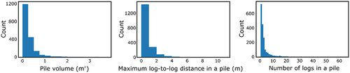
Figure 6. (a) The real-life graph created from a set of loading nodes and an estimate of the roadside delivery node location (gray dot) for system 4 (see Table 1) (b) Decomposition of the real-life graph into a disjoint set of region graphs.

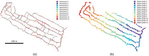
Figure 7. The first part of the algorithm for decomposing the real-life graph into a set of disjoint region graphs. In this part of the algorithm, the set of subgraphs, which will be used to create the decomposition in the second part of the algorithm, is formed and then ordered by increasing distance from the unloading node.

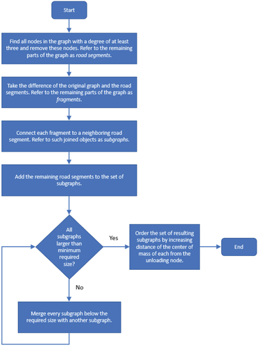
Figure 8. The second part of the algorithm for decomposing the real-life graph into a set of disjoint region graphs. In this part of the algorithm, the actual decomposition is constructed from the subgraphs created and ordered in the first part of the algorithm.

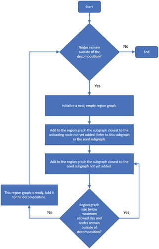
Figure 9. The static trafficability index for system 4 (see Table 1). The trafficability index is open data distributed by the Finnish Forest Centre (2020)

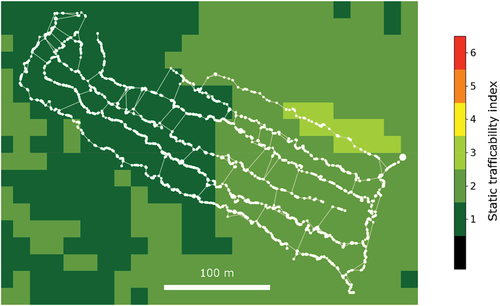
Figure 10. Optimized routes on the artificial model system. The solutions illustrate how the optimization algorithm separately minimizes distance, duration, and damage. The color of the arrow indicates the assortment of the destination node at each step of the route.

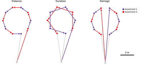
Figure 11. Artificial model system used to illustrate multi-objective optimization.

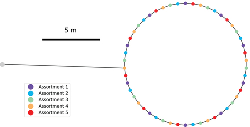
Table 2. Multi-objective optimization results for distance and duration on the artificial model system, and corresponding single-objective results for comparison.

Optimization criteria	Route length (m)	Duration (h)	Number of assortments in load
Distance	204.2	2.4	5
Distance and duration	230.5	1.9	3 to 4
Duration	275.6	1.5	2 to 3

Table 3. Essential parameter values used in optimizing the test system.

Parameter	Value
Forwarder loading capacity	12 m^3
Forwarder speed	1 m/s
$V_0$ in the ground damage model	10 m^3
$\rho$	0.01
$\alpha$	5
$\beta$	4
Number of ants	Number of loading nodes in the region graph
Length of candidate list	20
Number of ACO iterations	500

Table 4. Results for optimizing forwarder work in the test system using a single objective at a time. The best value for each metric is set in italics. Each result is an average over 10 randomly initialized optimizations. The error is the standard error of the mean.

Optimization criterion	Distance (km)	Duration (h)	Damage	Mean number of assortments in load
Distance	24.13 ± 0.07	30.28 ± 0.04	67,680 ± 120	4.63 ± 0.08
Duration	26.29 ± 0.07	28.48 ± 0.03	72,280 ± 140	4.16 ± 0.07
Damage	24.52 ± 0.07	30.54 ± 0.06	66,530 ± 100	4.67 ± 0.07

Figure 12. Example of a general view of optimized routes for a given region of the harvest site when minimizing total traveled distance. The arrows denote the order in which piles are picked up, with the color of the arrow indicating the assortment of the destination pile at each step along the route. Each transition between nodes (e.g., from the unloading node to the first node to be visited, i.e., pile to be loaded) is done along the shortest path on the strip road network. The long arrows denote transitions between the unloading node and the loading nodes.

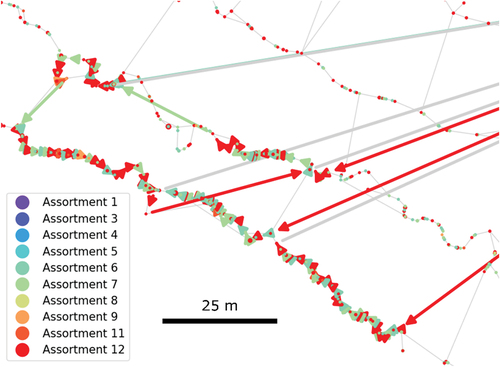
Figure 13. Close-up views of routes optimized considering only a single objective at a time: distance (a, b), duration (c), and soil damage (d). The arrows depict the route of the forwarder, with the color of the arrow indicating the assortment of the destination pile at each step of the route.

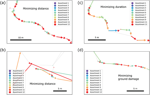
Figure 14. Convergence behavior of the optimization algorithm when optimizing one objective at a time. Each point is an average over 10 randomly initialized optimizations. The error is the standard error of the mean.

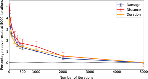
Figure 15. When minimizing ground damage, the optimized routes often displayed working patterns where the forwarder picks up piles while approaching the landing. This is a way of decreasing the total soil damage created.

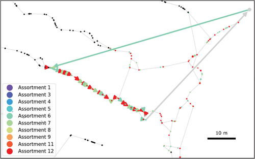
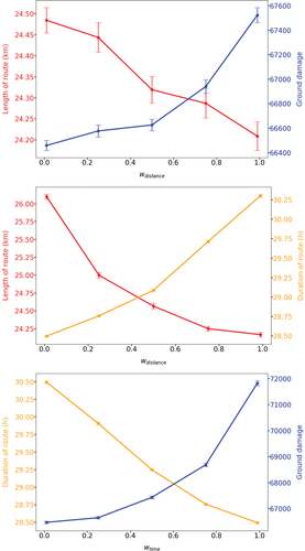
Figure 16. Results for optimizing two objective components at a time, using different values for the objective weights (Eq. 6)(6) $c\left(r\right)=w_{distance}\frac{D\left(r\right)}{\bar{D}}+w_{time}\frac{T\left(r\right)}{\bar{T}}+w_{damage}\frac{S\left(r\right)}{\bar{S}}$(6) . The weight (w) of the component plotted on the left vertical axis is given on the horizontal axis. The weight of the component plotted on the right vertical axis is equal to 1 – w. Each point is an average over 50 randomly initialized optimizations. The error is the standard error of the mean.

Finnish Forest Centre. 2020. Harvestability maps of Finland. [accessed 2020 Nov 20]. https://www.metsakeskus.fi/korjuukelpoisuuskartat.

 Google Scholar