
Figures & data
Figure 1. Input/output function for a frequency-compression hearing aid with Sf = 1 kHz and CR = 2. Frequency components below Sf remain unchanged. In this example, the high-frequency edge of the source band, Ef, is 4 kHz. The width of the source band in octaves is 3.32log10(Ef/Sf), which is 2 octaves. The width of the destination band is 3.32log10(Ef/Sf)/CR, which is 1 octave. Thus, its upper edge falls at 2 kHz.
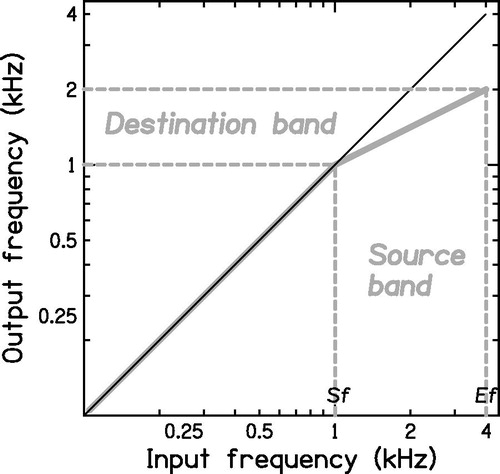
Table 1. Demographic data of the participants.
Figure 2. Air-conduction audiograms of the ears tested. Open circles and crosses indicate thresholds for the right and left ears, respectively. Down-pointing arrows indicate that the participant did not respond at the highest level tested.
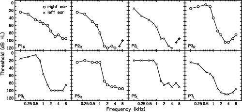
Figure 3. TEN(HL) test results. Audiometric thresholds measured as part of this test are shown using the same symbols as for . When the audiometric threshold was higher than the maximum tone level of 104 dB HL, the threshold is not shown. The level of the TEN(HL) in dB/ERBN is shown by the dashed lines without symbols. The masked thresholds of the tone in the TEN(HL) are shown by open squares. Downward-pointing arrows mean that the participant did not detect the tone at the level indicated. Shaded areas indicate frequencies where the outcome of the test was positive. Cross-hatched areas indicate frequencies where the outcome was inconclusive.
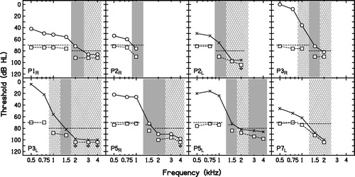
Figure 4. Examples of PTCs. The signal frequency and level are denoted by an open star. The dotted line shows the masker levels visited, and the continuous line shows the combination of an upward-sweep and a downward-sweep run, after smoothing each of them. The frequency at the tip of each PTC (the MMF) is indicated in each panel. The MMF was taken as the estimate of fe.
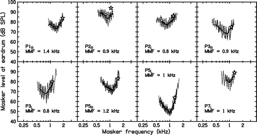
Figure 5. Fast PTCs for P5L. For fs = 1.3 kHz, the tip was shifted to 1 kHz. For fs = 3 and 3.5 kHz, the tips were shifted to 2.9 and 2.8 kHz, respectively. See the text for a discussion of these results.
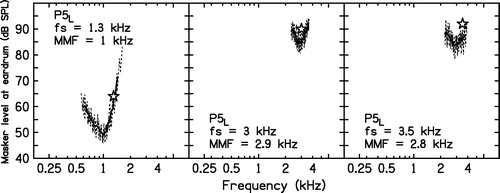
Figure 6. Mean quality ratings for P1R, P2R, P2L and P3R for each frequency-compression condition and for the control condition (C), plotted separately for each talker. Values of Sf and CR are shown at the top and bottom, respectively. Each row represents one ear. The error bars represent ±1 SD of the ratings after correction for order effects. For each ear, the leftmost panel shows the mean corrected ratings for the control condition when the reference stimulus was compared with itself, for the male talker (M) and the female talker (F). 95% confidence intervals were calculated from these ratings. Stars indicate that the mean ratings for a given frequency-compression condition were outside the 95% confidence intervals for the control condition.
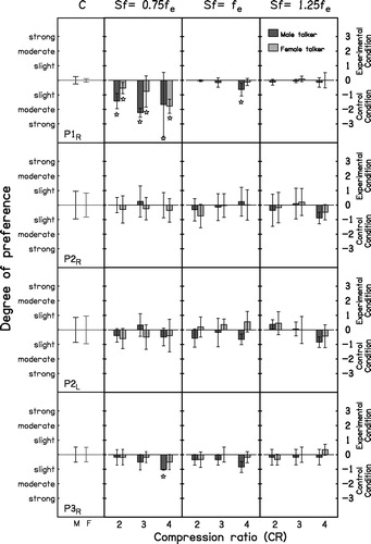
Figure 7. As , but for P3L, P5R, P5L and P7L.
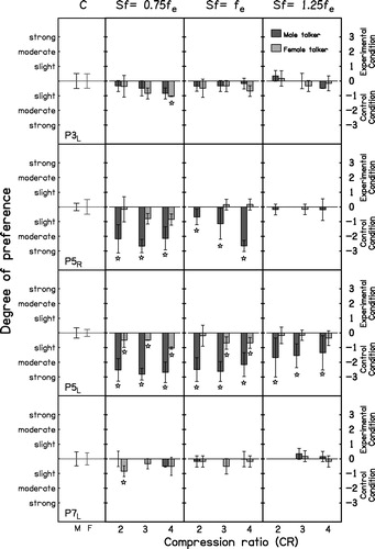
Table 2. Audibility calculations for P1R–P3R.
Table 3. As but for P3L–P7L.